
The views expressed in this paper are those of the writer(s) and are not necessarily those of the ARJ Editor or Answers in Genesis.
Abstract
The “Pacemaker of the Ice Ages” paper by Hays, Imbrie, and Shackleton convinced uniformitarian scientists of the validity of the modern version of the Milankovitch hypothesis of Pleistocene ice ages. Spectral analyses performed on three variables from two Indian Ocean sediment cores showed prominent spectral peaks with periods corresponding to dominant cycles in earth’s rotational and orbital motions. Yet there are serious problems with this iconic paper. The assumed age of 700 ka for the Brunhes-Matuyama (B-M) magnetic reversal boundary, used to help construct age models for the analysis, has since been revised significantly upward to 780 ka. Also, the paper’s authors may have needlessly excluded nearly one-third of all the available data from the second core. This paper discusses statistical significance and the manner in which these issues affect the original published results. These changes dramatically weaken—if not completely invalidate—the argument for the Milankovitch hypothesis presented in this paper, even if one excludes the disputed section of data from the second core. This conclusion has tremendously important implications for uniformitarian dating methods and the global warming/climate change debate.
Introduction
The Milankovitch hypothesis is the dominant explanation for the 50 or so Pleistocene “ice ages” which uniformitarian scientist claim to have occurred within the last 2.6 million years (Walker and Lowe 2007). Summaries of the hypothesis are provided in (Hebert 2014; 2015; 2016a). Despite its popularity, the hypothesis has many problems that are acknowledged even by secular scientists (Cronin 2010, 130–139).
Despite these difficulties, the hypothesis is generally seen as having been vindicated (and elevated to the status of theory) by a seminal 1976 paper in Science entitled “Variations in the Earth’s Orbit: Pacemaker of the Ice Ages” (Hays, Imbrie, and Shackleton 1976, hereafter referred to as Pacemaker). Hays, Imbrie, and Shackleton performed spectral analyses on three variables of presumed climatic significance within the two Indian Ocean sediment cores RC11-120 and E49-18 (fig. 1). Spectral analyses of oxygen isotope (δ18O) ratios of the planktonic foraminiferal species Globigerina bulloides, the relative abundance of the radiolarian species Cyclodophora davisiana, and (southern hemisphere) summer sea surface temperatures (also inferred from radiolarian data) revealed spectral peaks corresponding to periods close to 100, 41, and 23 ka. Since these periods correspond to major cycles in earth’s orbital and rotational motions, the Pacemaker paper is widely seen as providing strong support for Milankovitch climate forcing.
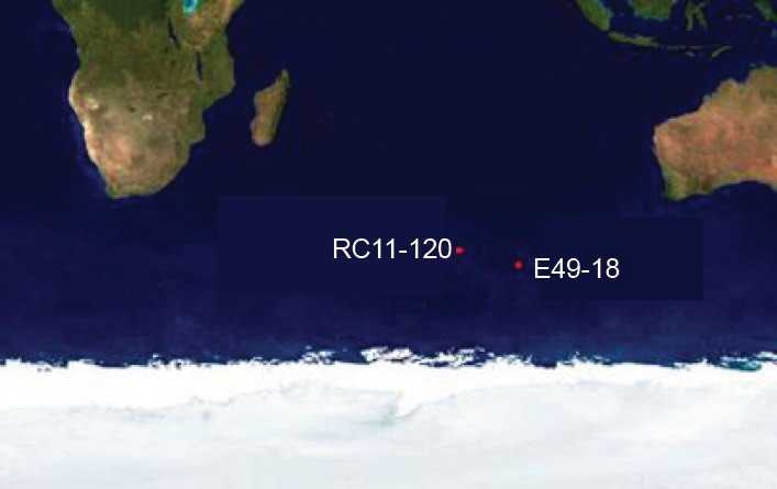
Fig. 1. The 1976 Pacemaker paper by Hays, Imbrie, and Shackleton used data from Indian Ocean deep-sea sediment cores RC11-120 and E49-18.
In particular, the Pacemaker authors used the Blackman-Tukey (1958) method to perform their spectral analyses of the RC11-120 and E49-18 data. For those unfamiliar with the Blackman-Tukey (B-T) method, a primer is given in Hebert (2016b).
However, this seminal paper suffers from a number of serious problems (Hebert 2016a). Before they could perform their spectral analyses, the Pacemaker authors had to construct age models for the two sediment cores. Critical to these age models was an assumed age of 700 ka for the Brunhes-Matuyama (B-M) magnetic reversal boundary (Hays, Imbrie, and Shackleton 1976, 1124, 1131; Shackleton and Opdyke 1973, 40). However, uniformitarian scientists have since revised this age upward to about 780 ka (Berger et al. 1995; Karner et al. 2002; Muller and MacDonald 2000; Shackleton, Berger, and Peltier 1990). This is by far the most serious problem with the paper, although it also suffers from other difficulties (Hebert 2016a).
The reader may wonder why this age revision and its possible impact on the Pacemaker results have been overlooked for so long. Quite simply, the Pacemaker paper never explicitly mentioned the age of the B-M reversal boundary, although it stated that the boundary was used to help construct the age models for the two cores (Hays, Imbrie, and Shackleton 1976, 1124). However, the Pacemaker paper referred to an earlier paper, which explicitly stated (Shackleton and Opdyke 1973, 40) the age of the B-M reversal boundary to be 700 ka. This age for the B-M reversal boundary was used to help construct the age models used in Pacemaker.
The methodology used in the Pacemaker paper and the revised age for the B-M reversal boundary introduces a potential “causality problem” in that it “pushes back” the ages for several ice age/interglacial transitions by multiple tens of thousands of years.
Furthermore, the Pacemaker authors excluded nearly a third of all the available data from the E49-18 sediment core, probably needlessly. These problems in the Pacemaker paper are discussed at greater length below.
Additional Problems: Core Discontinuities?
After publication of the first paper (Hebert 2016a) in this series, I found other potential problems with the Pacemaker paper. Uniformitarian scientists used western Pacific core V28-238 to assign ages to the first 21 marine isotope stage (MIS) boundaries. For those unfamiliar with the concept of MIS boundaries, a discussion is presented in Hebert (2016a). Uniformitarian scientists originally claimed that continuity of the V28-238 core was “virtually proved” (Emiliani and Shackleton 1974, 513) by very good correlation between its isotopic features and isotopic features within other cores. Because of this presumed continuity, uniformitarian scientists felt justified in assuming an approximately constant sedimentation rate within the V28-238 core and using the B-M magnetic reversal boundary to assign ages to the MIS boundaries (Shackleton and Opdyke 1973). For this reason, the isotope record within the V28-238 core has been described as a kind of ice age “Rosetta Stone” (Woodward 2014, 97). A number of these MIS boundary age assignments were used in the Pacemaker analysis (Hays, Imbrie and Shackleton 1976).
But uniformitarian scientists later claimed, on the basis of comparisons with still other cores, that the V28-238 core had been disturbed, particularly within marine isotope stages 5 and 11 (Imbrie et al. 1984; Prell et al. 1986).
Claims of core discontinuities are sometimes based, not upon prima facie evidence of disturbance, but rather upon “unexpected” oxygen isotope behavior. Because uniformitarian scientists believe that the δ18O signal is globally synchronous (Prell et al. 1986, 137), they are expecting the same identifiable marine isotope features to be present in all undisturbed cores. So the absence of expected δ18O features, or the presence of unexpected δ18O features, can be seen as evidence of a core disturbance, the influence of “local” weather/climate, or depositional effects. Of course, depending on which cores are used in the inter-core comparisons, one can make a case both for and against a discontinuity from the same section of the same core. This is evident from the contradictory claims discussed above regarding continuity in the V28-238 core.
However, in the case of the RC11-120 and V28-238 cores, there does seem to have been actual evidence that the cores were indeed disturbed (Imbrie et al. 1984, 282; Prell et al. 1986, 153). However, the uniformitarian consensus seems to be that a possible disturbance in Stage 5 within V28-238 was not too large; Prell et al. (1986, 149) did not even attempt to correct for it.
However, uniformitarian scientists did attempt to take into account a possible disturbance within V28-238’s Stage 11. As noted by Imbrie et al. (1984, 288), depths below 723 cm in V28-238 were reduced by 30 cm in order to take into account this possible core break. Since the original reported depth of the MIS 12-11 boundary within V28-238 was 755 cm (Shackleton and Opdyke 1973, 49), the revised depth for that boundary became 725 cm. Likewise, the new depth of the B-M reversal boundary became 1170 cm. Shackleton and Opdyke’s methodology, together with the currently accepted age of 780 ka for the B-M reversal boundary, yields a new estimated age of 780 ka × (725/1170) = 483 ka for the MIS 12-11 boundary. This is a little lower than the new age of 491 ka that one obtains without taking into account this possible core disturbance (Hebert 2016a, 33).
Since the 220cm depth of the MIS 6-5 boundary in V28-238 (Shackleton and Opdyke 1973, 49) is unchanged, the new age for the MIS 6-5 boundary becomes 780 ka×(220/1170)=147 ka, which is a little higher than the age of 143 ka that one obtains without taking into account this possible discontinuity (Hebert 2016a, 33).
Likewise, because the original depth of 430cm for the MIS 8-7 boundary would not need to be adjusted, the new age for this boundary would become 780 ka×(430/1170)=287 ka. This is about 7 ka older than the revised age that one obtains without taking into account this possible discontinuity, and 36 ka older than Shackleton and Opdyke’s original estimated age of 251 ka.
In re-performing the Pacemaker analysis, I have elected to ignore these possible discontinuities for the following reasons. First, the methodology used to correct for possible core discontinuities requires a technique that is beyond the scope of this paper (Prell et al. 1986; Shaw 1964). Adjustments to the timescales caused by these possible core discontinuities may be addressed in later works. However, the potential causality problems (discussed later in this paper) caused by the new age estimate for the B-M reversal are still present, regardless of whether one attempts to correct for potential discontinuities in the V28-238 core, or even in the RC11-120 and E49-18 cores.
A Complication: Negative Spectral Values
As noted earlier, the Pacemaker authors used the Blackman-Tukey (B-T) method to perform their analyses of the RC11-120 and E49-18 data. In the B-T method, the spectral power is the Fourier transform of the autocovariance of the data. For readers unfamiliar with the B-T method of spectral analysis, a primer is provided in Hebert (2016b). This primer also discusses bandwidth, null continua, confidence intervals, prewhitening, and statistical significance, concepts that are used extensively throughout this paper.
When using the B-T method, one is, in effect, numerically integrating the product of a cosine function and an autocovariance function. Since both the cosine function and the autocovariance function can be either positive or negative, the B-T method can sometimes yield negative values of spectral power, even though spectral power should theoretically be strictly non-negative. This is especially true at high frequencies in “red” spectra, as spectral powers at these high frequencies tend to be quite small anyway. In fact, these negative power values are usually present in the null continua more so than the power spectra per se. These negative values complicate things a bit, since researchers generally plot the natural logarithm of spectral power versus frequency when investigating the statistical significance of spectral peaks. Since one cannot take the natural logarithm of a non-positive number, these negative values must first be converted to positive values.
One method is to simply truncate these negative values to some very small positive value, say, 0.0001.
A second method is to determine the most negative power value from the power spectrum and the most negative power value from the null continuum and to choose the smaller (most negative) of those two numbers, taking the absolute value of the result. As in the previous method, since one cannot take the natural logarithm of zero, a very small constant, say 0.0001, is then added to this result. The resulting value is then added to each frequency-dependent spectral power, both for the power spectrum itself, and for the null continuum. This additive constant is then multiplied by the number of frequencies in the spectra and the resulting number is then added to the original calculated variance. After these steps, normalization is achieved as in the same manner when no negative spectral values are present. This “vertical offset” method essentially shifts both the spectrum and null continuum upward by the same amount.
A third method is to give greater weight to the l=0 term in Eq. (32) in Hebert (2016b), by changing the first “2” in the equation to a number greater than 2 and less than or equal to 4. This shifts slightly upward the “floor” of the power spectrum, with every frequency contributing a small amount of variance to the total variance of the signal. Careful choice of this constant can prevent negative values of spectral power. I personally prefer this option as it seems to be the least ad hoc and flows very naturally from the derivation of Eq. (32) that was presented in (Hebert 2016b), especially if one sets this constant to exactly 4.
Most of these negative spectral powers appear in the null continua rather than the power spectra per se, and the handful of negative spectral powers that do appear in the power spectra are generally extremely tiny. The Pacemaker authors did not explicitly state how they handled potentially negative spectral powers. It seems to have been a moot point for them, since they only plotted the null continua for their prewhitened spectra, which do not seem to have been subject to this complication (see the bottom row of their fig. 6). However, since I have chosen to plot the null continua for my unprewhitened spectra, I have to address this difficulty. I have chosen to use the truncation method because it seems to yield the best agreement between my replicated power values and those shown in Fig. 5 in the original Pacemaker paper, provided that one multiplies their power values by two, per the discussion in Hebert (2016b, 144). Also, in this particular case at least, truncation seems to yield results slightly more favorable to statistically significant peaks. Hence, I chose to truncate negative spectral powers, setting them equal to 0.0001.
Some reflection reveals why the truncation of negative values within the null continuum tends to favor the detection of statistically significant peaks more so than the vertical offset method. If fnum is the number of frequencies in the B-T spectrum, one can think of the unnormalized power values for the null continuum as a series of fnum numbers, most of which are positive, but a few which are slightly negative. Following Eq. (36) in Hebert (2016b), the sum of these fnum numbers is multiplied by a normalization constant and a frequency interval in order to ensure that the sum is equal to the variance of the original data set. Note that this normalization condition is also imposed on the power spectrum itself. Replacing the handful of negative power values within the sum with slightly positive power values will increase slightly the value of this sum. In order for the normalization condition to continue to hold true, the normalization constant for the null continuum must be slightly decreased, since the frequency interval does not change. If no negative spectral powers are present in the actual power spectrum, then the normalization constant for the power spectrum will be unchanged. Hence, the slight decrease in the null continuum’s normalization constant will cause the null continuum to be lowered slightly relative to the location of the power spectrum, enhancing somewhat the apparent statistical significance of a given spectral peak. Because most of the truncated values in this study were power values within the null continua rather than the power spectra themselves, this tended to slightly favor statistically significant results.
Replication of Original Prewhitened PATCH Results
I presented reproduced results from the original Pacemaker paper’s Fig. 5 in Hebert (2016b). Because the surviving Pacemaker authors did not respond to my requests for their data, I had to reconstruct the original 10 cm resolution data from Figs. 2 and 3 in the Pacemaker paper. These reproduced data values are found in the appendices of Hebert (2016a). The three charts in the first row of Fig. 6 of Pacemaker are basically equivalent to the three charts in the last row of their Fig. 5, except that the results in their Fig. 6 are depicted on a semi-log graph. Since I have already reproduced these three charts in Figs. 15–17 in Hebert (2016b), reproducing the first row of their Fig. 6 would be redundant. However, I also reproduced the results from the second row of their Fig. 6, using my reconstructed data values and the ELBOW chronology they assigned to the PATCH “core.” PATCH was not a real core but was a data set constructed by joining data values in the top 785 cm of the RC11-120 core with the data values found below 825 cm in the E49-18 core (see the caption for their table 2).
In Figs. 2–4 each PATCH power spectrum is plotted against frequency on a semi-log graph. As in the original Pacemaker paper, these results were all obtained with Δt = 3 ka, which implies that the number of interpolated data points n is 163 (but n is reduced by one during the prewhitening process). Likewise, the power spectra were obtained, as in the original Pacemaker paper, with m set to 50; the meaning of this index is discussed in Hebert (2016b, 135–137). The thick red lines are the null continua. The Pacemaker authors obtained their null continua for all three PATCH spectra by setting m equal to 8 (Hays, Imbrie, and Shackleton 1976, 1132, reference #57), but my results seem to agree better with theirs if I use m = 7. The thin green and blue lines are the bounds of the 80% and 90% confidence intervals, respectively, and the blue bracket is the approximate bandwidth. Note that in the following figures, the width of the blue bracket may disagree slightly with the bandwidth value calculated from Eq. (35) in Hebert (2016b), due to resolution limitations.
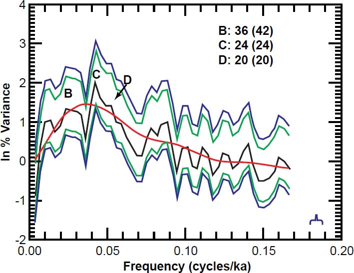
Fig. 2. Natural log of my replicated PATCH power spectrum for the prewhitened SST data, plotted as a function of frequency. The red curve is the null continuum, the green and blue lines are the bounds of the 80% and 90% confidence intervals, respectively, and the blue bracket is the bandwidth. Numbers in bold are the periods (in ka) of the dominant peaks, while the numbers in parentheses are the periods for those peaks reported in the Pacemaker paper.
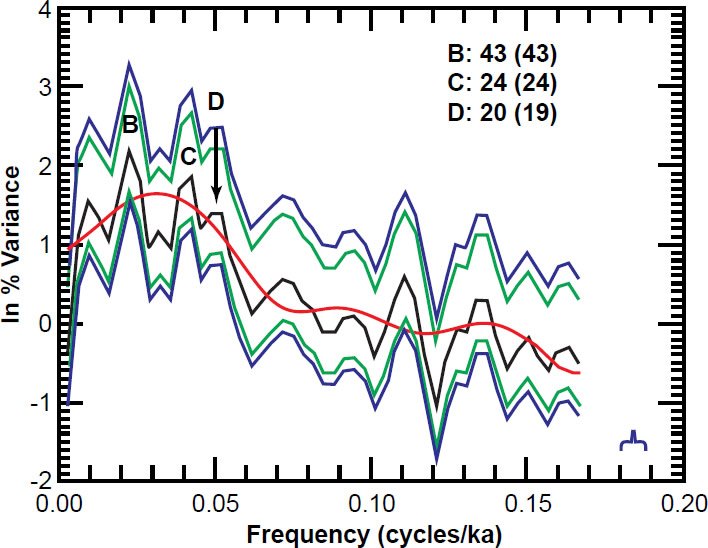
Fig. 3. Natural log of my replicated PATCH power spectrum for the prewhitened δ18O data, plotted as a function of frequency. The red curve is the null continuum, the green and blue lines are the bounds of the 80% and 90% confidence intervals, respectively, and the blue bracket is the bandwidth. Numbers in bold are the periods (in ka) of the dominant peaks, while the numbers in parentheses are the periods for those peaks reported in the Pacemaker paper.
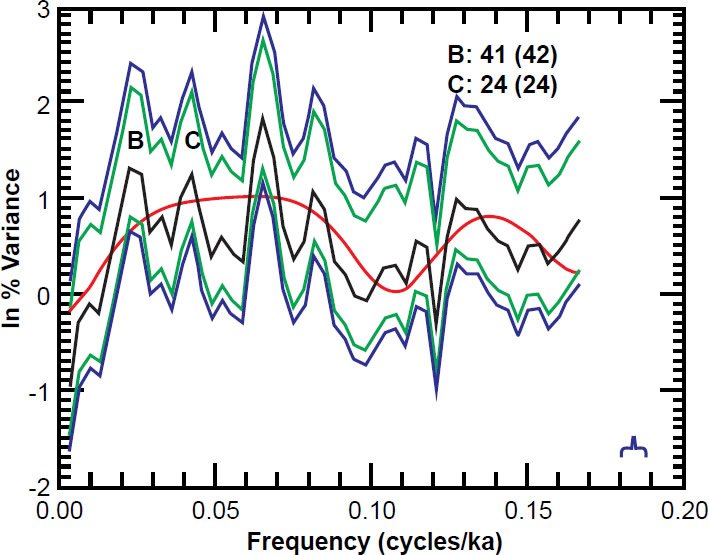
Fig. 4. Natural log of my replicated PATCH power spectrum for the prewhitened % C. davisiana data, plotted as a function of frequency. The red curve is the null continuum, the green and blue lines are the bounds of the 80% and 90% confidence intervals, respectively, and the blue bracket is the bandwidth. Numbers in bold are the periods (in ka) of the dominant peaks, while the numbers in parentheses are the periods for those peaks reported in the Pacemaker paper.
Since the width of a particular confidence interval does not vary with frequency on a semi-log graph (Jenkins and Watts 1968, 255), many authors prefer to indicate the width of a confidence interval with a single arrow somewhere on the semi-log graph. However, I have elected to explicitly show the bounds of my confidence intervals, partly because this makes it easier to determine at a glance if a given peak is statistically distinguishable from the background.
In order to be as charitable as possible to the original Pacemaker paper, I have set the number of degrees of freedom v equal to 2.516n/m rather than 2n/m (the expression used by the Pacemaker authors), per the discussion in Hebert (2016b, 140–141). The Pacemaker authors used a prewhitening constant of C=0.998 (see their fig. 6), but I set my value of C to the maximum value of 0.999 (Imbrie and Pisias n.d., 9). Such a tiny difference in the value of C will not noticeably affect the results, and it seems odd that the Pacemaker authors did not simply set C to the maximum possible value.
The numbers on the vertical axes do not agree with those in the Pacemaker paper for a number of reasons. The ambiguity in how the Pacemaker authors handled potentially negative spectral values made it more difficult to precisely match numbers on the vertical axis, as did subtle differences in the heights of our spectral peaks, even after taking into account the factor-of-two difference in spectral power. Frankly, I did not think it worth the effort to try to “reverse engineer” their precise normalization constants. However, the choice of normalization constant is not critical, since the natural logarithm of a product is equal to the sum of the natural logarithms. Hence, a disagreement in normalization constants will simply shift the natural logarithms of both the power spectrum and the null continuum up or down by a constant value. Matching the actual numbers on the vertical axes is not what is important; rather, it is important to match the shapes of the spectral peaks and null continua, and the frequencies of the dominant spectral peaks.
After prewhitening, half the ~41 and ~23 ka peaks are statistically distinguishable from the null continuum, but only for 80% confidence intervals. For the δ18O B peak in Fig. 3, the lower bound of the 90% confidence interval is just slightly below the null continuum. The same is true for the % C. davisiana B peak in Fig. 4; the left edge of the 90% confidence interval is just below the null continuum). Generally, my spectral peaks are wider and less pronounced than in the original Pacemaker paper. Since the differencing process used to prewhiten the data is analogous to taking the derivative of the original data set (Muller and MacDonald 2000, 95), subtle errors in my reconstruction of the original data are amplified by prewhitening, as well as by the depiction on a semi-log graph.
Overall, the shapes of the null continua in Figs. 2–4 agree fairly well with the null continua shown in the bottom row of Fig. 6 in Pacemaker, with the possible exception of a dip in the % C. davisiana null continuum around 0.11 cycles/ka that is much more pronounced in my Fig. 4 than in the original Pacemaker paper. However, closer inspection reveals that this discrepancy may be more apparent than real: the Pacemaker authors compressed the vertical scale (bottom right corner of their Fig. 6), not “filling up” all the available space that was available. This would have the effect of causing this dip to appear shallower in their chart than it appears in my Fig. 4.
The number in bold corresponding to each B, C, or D peak is the period of the corresponding cycle in ka. Numbers in parentheses indicate the periods originally reported in Pacemaker. In order to obtain the best possible visual matches to the original results, I used m+1 discrete frequencies for the depicted results, as indicated by the Pacemaker authors (Hays, Imbrie, and Shackleton 1976, 1132). However, in order to obtain more precise frequency/ period estimates, I re-did the calculations using an increased number (3m) of frequencies. In most cases, these higher resolution spectra made it relatively easy to determine the frequency/period corresponding to each peak. In the cases in which a single highest spectral power for the peak was not obvious (say, because the central frequency of the peak fell between two plotted power values), I obtained an average of the handful of (usually two) frequencies in the vicinity of the peak, weighted by the spectral power at each of the individual frequencies near the peak.
Prominent peaks are present near the expected frequencies, although the peaks are not as pronounced as those in the original Pacemaker paper. Also, the agreement between my replicated PATCH results and the original reported results is poorer than the agreement between my results for their Fig. 5 (Hebert 2016b), particularly in the high-frequency region of the spectrum. As already noted, this is likely the result of subtle errors in my reconstructed data values, due to the difficulty of reading data values off their Figs. 2 and 3. These errors will be amplified even more on a semi-log plot.
The point of this exercise was to demonstrate that I can reproduce the results from the second row of Fig. 6 in the Pacemaker paper with a reasonable degree of precision. Of course, these results are all moot, as they were obtained using an assumed age of 700 ka for the Brunhes-Matuyama magnetic reversal, an age no longer accepted by uniformitarian scientists. Of far greater interest is the effect that this revised age, as well as the inclusion of data from the top portion of the E49-18 core, has on the original Pacemaker results. However, before discussing this issue, it is necessary to discuss a number of other issues related to the Pacemaker paper.
Spectrum Blurring: An Additional Constraint
In order to determine whether the periods of the orbital (eccentricity, obliquity, and precession) cycles obtained from their spectra agree with the periods obtained from the geological (δ18O, SST, and % C. davisiana) spectra, one must obtain orbital power spectra specifically for the time interval under consideration. This is because the orbital cycles are quasi-periodic: although they tend to have periods of around 100, 41, and 23 ka, the actual values of the periods depend upon the precise time interval under consideration. This is especially true for the eccentricity and precessional cycles. Hence, the theoretically expected frequencies/periods should be obtained from orbital spectra calculated specifically for the time interval corresponding to each particular trial (Muller and MacDonald 2000, 33, 36).
In performing my orbital calculations, I obtained my period estimates from spectra of the calculated orbital parameters of Berger and Loutre (1991), which, as of 6/17/2016, were archived at https://doi.pangaea.de/10.1594/PANGAEA.56040?format=html#lcol0.ds1004521. These newer calculated values are more accurate than an earlier set (Berger 1978), which were quite inaccurate for times more than 1.5 million years ago (Muller and MacDonald 2000, 29) due to a round-off error (Quinn, Tremaine, and Duncan, 1991). Although the original Pacemaker paper used the earlier calculated set of orbital parameters, one does not expect there to be much difference between the old and new results, since even the 1978 values should be reasonably accurate for the relatively “recent” times used in the Pacemaker paper.
This discussion implies an additional constraint when comparing theoretical with experimental results. Such a comparison can only be made for orbital elements whose periods may be estimated from the relevant power spectra for a given value of m. For relatively small values of m, a clear eccentricity peak may not be apparent at f~0.01 cycles/ka. In that case, one cannot make a comparison between the experimentally determined low frequency “A” periods from the geological spectra and the ~100 ka eccentricity period predicted from Milankovitch expectations. Moreover, the time interval also needs to be sufficiently long that one could reasonably estimate the long eccentricity period; for instance, the Pacemaker authors only made a comparison between the eccentricity period and the periods of the A geological peaks for their long ELBOW chronology applied to the PATCH “core.”
In the following analyses, I “follow their lead” and only calculate eccentricity periods for the two trials characterized by time intervals greater than 500 ka. However, I do calculate obliquity and precession periods for all the trials, so that their periods may be compared to the periods of the B and C peaks in the geological spectra.
These astronomical periods should also be calculated with the Blackman-Tukey method, using the same degree of blurring applied to the geological spectra of each trial. At first, one might suspect that such blurring of the orbital spectra would be inappropriate, since one of the justifications for blurring geological spectra, possible changes in sedimentation rate (Muller and MacDonald 2000, 16, 63–66), is not an issue for orbital motions. However, two other issues must be considered. First, orbital spectra have very narrow spectral peaks, since astronomical processes experience low energy losses (Muller and MacDonald 2000, 21). Likewise, if astronomical processes are influencing climate, one expects the resulting geological spectra to also have narrow peaks (Muller and MacDonald 2000, 19–28). But in the Blackman-Tukey method, the apparent width of a spectral peak also depends upon the degree of blurring, which is controlled (for a given value of n) by the choice of the parameter m. Smaller values of m tend to “blur” the spectrum more, causing the peaks to be wider. Second, in some cases, orbital spectra show eccentricity and precessional “doublets” consisting of two closely spaced spectral peaks. Closely spaced narrow peaks may “merge” into a single broad peak if a small enough value of m is used for the analysis. Hence, whether one expects to observe a doublet of closely spaced narrow peaks or a single broad peak depends on the value of m chosen for the analysis. Hence a fair comparison between geological and orbital spectra requires that both the orbital and geological spectra be blurred by the same amount.
This discussion raises a related puzzling issue. Based on their spectral analysis, the Pacemaker authors seemed to be saying that the eccentricity period over the interval 0 to 486 ka is 105 ka (see their table 4). Actually, it seems the authors transposed the “8” and “6” in “486,” as they actually stated that the period was obtained for the interval 0 to 468 ka. However, the correct time interval is clearly 486 ka, as the time interval for the interpolated PATCH data, Δt=3 ka, divides evenly into 486 ka, but not into 468 ka.
The caption to their Table 4 seems to imply that, for this particular trial, they used n=163 and m=50 to estimate the astronomical periods, just as they did for the three geological spectra. However, when I tried to replicate these results using Berger’s 1978 eccentricity values (obtained from the Goddard Institute for Space Studies, http://data.giss.nasa.gov/ar5/srorbpar.html) and those same values of n and m, no clear eccentricity peak is apparent at ~0.01 cycles/ka (fig. 5). In order to discern the ~100 ka peak, one needs to use a larger value of m. Hence, it is not clear how the Pacemaker authors obtained this particular result, as they did not elaborate on their procedure. Of course, this is all moot, anyway, as they obtained those results using an age for the Brunhes-Matuyama magnetic reversal that uniformitarian scientists no longer accept.
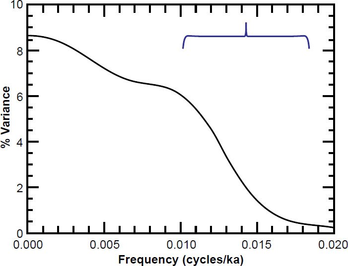
Fig. 5. Close-up of the low frequency part of the eccentricity power spectrum (calculated for 0 to 486 ka using Berger’s 1978 values). Spectrum was obtained using the Blackman-Tukey method, with n = 163, m = 50, and Δt = 3 ka. Blue bracket is the bandwidth.
Pacemaker Problem: The Age Revision for the Brunhes-Matuyama Magnetic Reversal Boundary
At this point, it is worthwhile to review the problems that the new age of 780 ka for the Brunhes-Matuyama (B-M) magnetic reversal boundary introduces to the Pacemaker results (Hebert 2016a). The Pacemaker authors used an assumed age of 700 ka for the B-M reversal boundary, plus the assumption of an approximately constant sedimentation rate within the V28-238 western Pacific sediment core, to assign tentative ages to the first 21 marine isotope stage (MIS) boundaries (Shackleton and Opdyke 1973). Three of these ages played a direct or indirect role in Pacemaker: an age of 128 ka for the MIS 6-5 boundary, an age of 251 ka for the MIS 8-7 boundary, and an age of 440 ka for the MIS 12-11 boundary.
Hays, Imbrie, and Shackleton did not make direct use of the 128 ka age for the MIS 6-5 boundary. Rather they used an age of 127 ka obtained from 231Pa–230Th dating of the Caribbean sediment core V12-122, as they considered this slightly younger age to be more trustworthy (Broecker and van Donk 1970, 173; Hays, Imbrie, and Shackleton 1976, 1124). They no doubt, however, considered the close agreement between the ages obtained from these two different methods as a confirmation of the validity of their assumption of a constant sedimentation rate in the V28-238 core.
They then used these ages (127 ka, 251 ka, and 440 ka) to construct the age models for the two cores prior to performing their spectral analyses. In their SIMPLEX age models, they only used the age estimates of 127 ka and 440 ka, but they used all three ages when constructing the ELBOW age model for the PATCH “core.”
This revised age of 780 ka for the B-M magnetic reversal boundary introduces an apparent discordance for their estimated ages for the MIS 6-5 boundary. Application of the exact same procedure used by Shackleton and Opdyke (1973), but with an age of 780 ka for the B-M reversal boundary, results in an estimated age of 143 ka for the MIS 6-5 boundary. Furthermore, as we have already noted, a possible discontinuity in the V28-238 core would raise this age estimate to 147 ka. This immediately raises a question: which, if either, of the two age estimates for the MIS 6-5 boundary should be believed? Is the correct age 127 ka, or 143–147 ka? Or are the uncertainties large enough that they could both be correct?
In the most widely accepted version of the Milankovitch hypothesis, changes in high-latitude northern hemisphere summer sunlight pace the ice ages. This high-latitude summer insolation is thought to have just begun to increase 135 ka ago, but at that time it still would have been too weak to begin ending the second-to-last ice age (Karner and Muller 2000, 2144). This is not a problem, however, since the MIS 6-5 boundary is the supposed midpoint of this glacial-to-interglacial transition, and an age of 127 ka for that boundary still places that transition after the increase in sunlight that supposedly caused it. But an age of, say, 143 ka for the MIS 6-5 boundary (also known as Termination II) implies that this glacial interval was already ending ~10,000 years before the increases in high-latitude summer insolation that supposedly caused that glacial interval to end (Shakun et al. 2011, 1). Whether this causality problem is real, rather than merely apparent, will depend upon the uncertainties in the age estimates obtained from Shackleton and Opdyke’s method. Estimating these uncertainties may require Monte Carlo simulations, which are beyond the scope of this paper.
Lisiecki and Raymo (2005) obtained orbitally tuned age estimates for MIS boundaries using a benthic δ18 O sediment stack. As of 6/09/2016, these age estimates, which were tuned to a simple ice model based on June 21 insolation at 65°N, were archived at http://www.lorraine-lisiecki.com/LR04_MISboundaries.txt. They placed the MIS 6-5 boundary (Termination II) at 130 ka, the MIS 8-7 (Termination III) boundary at 243 ka and the age of the MIS 12-11 (Termination V) boundary at 424 ka. These last two values are fairly close to Shackleton and Opdyke’s (1973) original respective age estimates of 251 and 440 ka, but re-performing Shackleton and Opdyke’s calculations using the revised age for the B-M magnetic boundary implies ages of 280 and 491 ka, which are significantly greater than Lisiecki and Raymo’s age estimates for those events.
I compare in Table 1 the tuned age estimates for the first 21 MIS boundaries with the ages implied by Shackleton and Opdyke’s method, for assumed ages of both 700 ka and 780 ka for the B-M reversal boundary. For the MIS boundaries represented in the RC11-120 and E49-18 cores, none of Shackleton and Opdyke’s original age estimates differed from Lisiecki and Raymo’s tuned age estimates by more than 16 ka, and most differences were not larger than 7 ka. Hence, the original age estimates for at least the 12 most recent MIS boundaries were in fairly good agreement with orbital tuning expectations. However, an assumed age of 780 ka for the B-M reversal boundary would have Terminations III, IV, and V occurring, respectively, 37 ka, 50 ka, and 67 ka before the times predicted for those events by Milankovitch climate forcing. If one believes that the age estimates derived from the V28-238 core have fairly small uncertainties, which would seem to be an implicit assumption in the Pacemaker analysis, then this would be a fatal objection to the Milankovitch theory, due to both the large sizes of the discrepancies and the potential causality problems implied by these discrepancies.
Moreover, Terminations VI and VII, which were not represented in the two Indian Ocean cores, occur respectively, 26 and 39 ka before the dates predicted by Milankovitch expectations. Although the MIS boundary ages implied by an age of 780 ka for the M-B reversal boundary do reduce the overall disagreement (based on a least squares analysis) between the tuned and untuned age estimates for all 21 MIS boundaries, the 12 MIS boundaries represented within the RC11-120 and E49-18 cores generally fare much worse with the newer timescale. Moreover, at least the age estimates based on an assumed age of 700 ka for the M-B reversal boundary do not place the glacial terminations long before the increases in summer solar insolation that supposedly triggered them.
I also took into account the effect that the correction for the possible stage 11 discontinuity in the V28-238 core (Imbrie et al. 1984, 288) would have on these calculated ages (remember that depths below 723cm were decreased by 30cm), and the results are shown in Table 2. Again, the revised age for the B-M reversal boundary greatly worsens the discrepancies between the two different age estimates for the MIS boundaries represented in the RC11-120 and E49-18 sediment cores.
If one is going to re-do the Pacemaker spectral analysis, taking into account the new age of the B-M reversal boundary, he would be well-advised to first use only chronological anchor points that were not tied to the age of the B-M reversal boundary. This would “dodge” any potential causality problems caused by the new age of that boundary. Of course, it may not be possible to exclude those anchor points and yet to still obtain results consistent with Milankovitch expectations, but for uniformitarians hoping to salvage the original Pacemaker results, they should attempt to do this first, before performing spectral analyses using anchor points tied to this reversal boundary.
| MIS Boundary | Depth in V28-238 (cm) | S&O Age (ka) | Hebert Age (ka) | L&L Tuned Age (ka) | Old Difference (ka) | New Difference (ka) |
|---|---|---|---|---|---|---|
| 1-2 (TI) | 22 | 13 | 14 | 14 | 1 | 0 |
| 2-3 | 55 | 32 | 36 | 29 | -3 | -7 |
| 3-4 | 110 | 64 | 72 | 57 | -7 | -15 |
| 4-5 | 128 | 75 | 83 | 71 | -4 | -12 |
| 5-6 (T II) | 220 | 128 | 143 | 130 | 2 | -13 |
| 6-7 | 335 | 195 | 218 | 191 | -4 | -27 |
| 7-8 (T III) | 430 | 251 | 280 | 243 | -8 | -37 |
| 8-9 | 510 | 298* | 332 | 300 | 3 | -32 |
| 9-10 (T IV) | 595 | 347 | 387 | 337 | -10 | -50 |
| 10-11 | 630 | 368* | 410 | 374 | 7 | -36 |
| 11-12 (T V) | 755 | 440 | 491 | 424 | -16 | -67 |
| 12-13 | 810 | 473* | 527 | 478 | 5 | -49 |
| 13-14 (T VI) | 860 | 502 | 559 | 533 | 31 | -26 |
| 14-15 | 930 | 543* | 605 | 563 | 21 | -42 |
| 15-16 (T VII) | 1015 | 592 | 660 | 621 | 29 | -39 |
| 16-17 | 1075 | 627 | 699 | 676 | 49 | -23 |
| 18 | 1110 | 648* | 722 | 712 | 65 | -10 |
| 18-19 | 1180 | 688 | 767 | 761 | 73 | -6 |
| 20 | 1210 | 706 | 787 | 790 | 84 | 4 |
| 20-21 | 1250 | 729 | 813 | 814 | 85 | 2 |
| 22 | 1340 | 782 | 871 | 866 | 84 | -5 |
Likewise, uniformitarians should not “mix and match” age control points that were tied to the B-M reversal with age control points that were not. First, if one is willing to accept age estimates for the MIS8-7 and 12-11 boundaries obtained using Shackleton and Opdyke’s method (and the revised age of the B-M reversal boundary), there is no good reason not to also accept the age of the MIS 6-5 boundary obtained with the same method. Second, the new age for the B-M reversal boundary will stretch the timescales for the RC11-120 and E49-18 cores, as discussed in Hebert (2016a). Because the peak period estimates in the original Pacemaker paper were generally in good agreement with Milankovitch expectations, the new timescales will cause these period estimates to become higher, possibly making them inconsistent with Milankovitch expectations. But “mixing and matching” the 127 ka age estimate (which was not tied to the B-M reversal boundary) with the 491 ka age estimate (which was) would stretch the timescale for the bottom section of the E49-18 core even more.
For instance, the original SIMPLEX timescale assigned a total length of time of 363 ka to the bottom two-thirds of the E49-18 core. Using the new age estimates of 143 ka and 491 ka for the MIS 6-5 and 12-11 boundaries would stretch the length of this SIMPLEX timescale to 403 ka. But using the age of 127 ka for the MIS 6-5 boundary, along with the age of 491 ka for the MIS 12-11 boundary, would stretch this timescale to 421 ka. The more the timescale is stretched, the more the period estimates for the dominant peaks will also be stretched, and the more likely it becomes that those period estimates will contradict Milankovitch expectations.
Therefore, when re-doing the Pacemaker analysis, I will attempt to be charitable to the Milankovitch theory and will only use the 127 ka age estimate for the MIS 6-5 boundary in spectral analyses that do not use the MIS 8-7 and 12-11 boundaries as chronological anchor points.
| MIS Boundary | Depth in V28-238 (cm) | S&O Age (ka) | Hebert Age (ka) | L&L Tuned Age (ka) | Old Difference (ka) | New Difference (ka) |
|---|---|---|---|---|---|---|
| 1-2 (TI) | 22 | 13 | 15 | 14 | 1 | -1 |
| 2-3 | 55 | 33 | 37 | 29 | -4 | -8 |
| 3-4 | 110 | 66 | 73 | 57 | -9 | -16 |
| 4-5 | 128 | 77 | 85 | 71 | -6 | -14 |
| 5-6 (T II) | 220 | 132 | 147 | 130 | -2 | -17 |
| 6-7 | 335 | 200 | 223 | 191 | -9 | -32 |
| 7-8 (T III) | 430 | 257 | 287 | 243 | -14 | -44 |
| 8-9 | 510 | 305 | 340 | 300 | -5 | -40 |
| 9-10 (T IV) | 595 | 356 | 397 | 337 | -19 | -60 |
| 10-11 | 630 | 377 | 420 | 374 | -3 | -46 |
| 11-12 (T V) | 725 | 434 | 483 | 424 | -10 | -59 |
| 12-13 | 780 | 467 | 520 | 478 | 11 | -42 |
| 13-14 (T VI) | 830 | 497 | 553 | 533 | 36 | -20 |
| 14-15 | 900 | 538 | 600 | 563 | 25 | -37 |
| 15-16 (T VII) | 985 | 589 | 657 | 621 | 32 | -36 |
| 16-17 | 1045 | 625 | 697 | 676 | 51 | -21 |
| 17-18 (T18) | 1080 | 646 | 720 | 712 | 66 | -8 |
| 18-19 | 1150 | 688 | 767 | 761 | 73 | -6 |
| 19-20 (T20) | 1180 | 706 | 787 | 790 | 84 | 3 |
| 20-21 | 1220 | 730 | 813 | 814 | 84 | 1 |
| 21-22 (T22) | 1310 | 784 | 873 | 866 | 82 | -7 |
On the other hand, one could assume that the age estimate of 143 ka for the MIS 6-5 boundary is correct, rather than the age estimate of 127 ka, despite the resulting potential causality problems. I explore both possibilities in this analysis.
Pacemaker Problem: Needlessly Excluded Data?
There is reason to suspect that the Pacemaker authors needlessly excluded the upper third of the data from the E49-18 core. They claimed that the core top had been disturbed and was possibly as old as 60,000 years (Hays, Imbrie, and Shackleton 1976, 1123). If the core top were indeed that old, then it presumably would have been difficult to obtain a reliable radiocarbon date for the core top. In that case, their exclusion of these data would have been justified. However, the Pacemaker authors still could have tried to confirm or falsify their assertion of a great age for the core top by at least attempting to radiocarbon date it. To the best of my knowledge, they did not, nor have any uniformitarian scientists attempted to do so. Don’t uniformitarian scientists want to know the true age of this core top?
In fact, the Pacemaker authors did not even bother to plot the upper 3.5 meters’ worth of δ18O data on their Fig. 3! This was an especially serious omission in light of the fact that uniformitarian scientists believe that the δ18O signal is globally synchronous (Prell et al. 1986, 137). Remember that uniformitarian scientists expect the uppermost δ18O values in an undisturbed core to trend “upward” toward noticeably lower δ18O values, corresponding to warmer interglacial conditions. Hence they expect the most recent δ18O values to trend “upward” as they do in the RC11-120 core (Fig. 6a), with a possible slight “downward” dip at the very top. Now that Howard and Prell (1992) have measured and reported the uppermost E49-18 δ18O values, we can see that there is a significant “upward” trend in δ18O values at the (apparent) top of the E49-18 core (Fig. 6b). This trend is “truncated” compared to the trend in RC11-120, as these δ18O values do not “level off” as they do in RC11-120. A uniformitarian might very well interpret this to mean that the uppermost part of E49-18 was indeed scoured away by bottom currents, but he might also conclude, as did Howard and Prell (1992, 87, 91) that the uppermost section of the E49-18 core was still quite young. In that case, the top of the E49-18 core could potentially have been radiocarbon-dated within a uniformitarian framework. A recent radiocarbon date for the top of the E49-18 core would have provided the Pacemaker authors with an additional chronological anchor point, but it would also have implied that exclusion of data from the upper third of E49-18 was unwarranted.
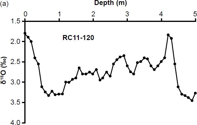
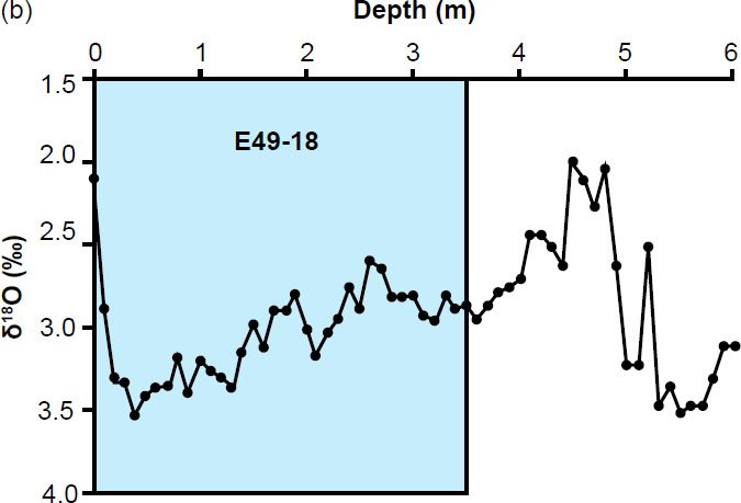
Fig. 6. Both the uppermost (a) RC11-120 and (b) E49-18 δ18O values trend “upward” toward more negative values. Because of the similarities between the two graphs, a uniformitarian scientist might conclude that the uppermost E49-18 δ18O values were of recent age and could potentially be radiocarbon dated. In that case, those data could have been used in the Pacemaker analysis. However, because the Pacemaker authors did not plot the uppermost E49-18 δ18O values on their Fig. 3, readers were denied the opportunity to judge for themselves whether or not this exclusion of data was reasonable. Shaded blue region in (b) indicates the δ18O data points omitted from Fig. 3 in the original Pacemaker paper.
But because the Pacemaker authors did not plot those δ18O values on their Fig. 3, readers of the original Pacemaker paper (not to mention the paper’s referees!) were denied the opportunity to judge for themselves whether this exclusion of data was reasonable. Naturally, this raises a question: what effect would inclusion of the uppermost 4.9m of E49-18 data have on the spectral results?
New Sedimentation Rates
Before re-performing the Pacemaker analysis taking into account this age revision and inclusion of these additional E49-18 data, it is important to check to make sure that the new calculated sedimentation rates will be sufficiently high for spectral analysis. At a bare minimum, one needs at least two sample data points per the smallest cycle that one is hoping to detect. Ideally, one would like to have more than this, say four, or preferably eight, data points per this smallest cycle (Weedon 2003, 35, 36). For a cycle of length 23 ka, eight data points per cycle would imply a sampling interval Δt=23 ka÷(8−1)=3.29 ka. If the data points are being sampled at 10cm intervals, as in the Pacemaker paper, this would imply a minimum sedimentation rate of 10cm÷3.29 ka=3.04cm/ka. However, a more lenient requirement of only 7 data points per cycle would allow the 23 ka cycle to be detected in cores with sedimentation rates as low as 2.61 cm/ka. For the cases discussed below, the new calculated average sedimentation rates prior to interpolation (which was deliberately kept to a minimum) were 4.26 cm/ka, 3.08 cm/ka, 2.63 cm/ka, 2.80 cm/ka, and 2.93 cm/ka. Hence, one does expect even the 23 ka cycle, if present, to “show up” in the following spectral analyses.
Testing Milankovitch: Criteria for Success
Before re-performing this analysis, one must have some way of determining whether the location of a spectral peak is in agreement with Milankovitch expectations, and this method should take into account the uncertainty Δf in the frequency of the peak.
The Pacemaker authors claimed their results confirmed Milankovitch climate forcing, in part because the frequencies of their B and C peaks within the RC11-120 and E49-18 SIMPLEX spectra agreed to within 5% of the calculated obliquity and precession frequencies (Hays, Imbrie, and Shackleton 1976, 1127). Actually, some of their calculated frequencies for the B and C peaks did not fall within these ranges. For instance, none of the frequencies for the RC11-120 B peaks fell within 5% of their reported frequency target values, nor did the frequency for the E49-18 δ18O B peak. Likewise, the frequencies for the RC11-120 SST C and the E49-18 SST and δ18O C peaks all fall just a little outside this 5% margin of error. Hence, this claim of 5% agreement by the Pacemaker authors is rather puzzling. Nevertheless, we will be using their “5%” criterion to evaluate the following results. The Pacemaker authors did not impose this same requirement on the 100 ka eccentricity cycle, possibly because the relatively short lengths of the RC11-120 and E49-18 core sections made precise determination of the frequency/period for the long eccentricity cycle more difficult.
A less stringent test would involve estimating the uncertainty Δf in the width of the spectral peak. This uncertainty will be on the order of the peak’s half-width at half-maximum (HWHM), but whether or not Δf is larger or smaller than the HWHM will depend on the local signal-to-noise ratio. However, for symmetrically shaped peaks, Δf is often taken to be, as a first approximation, plus or minus the HWHM. Or equivalently, the frequency of a spectral peak is only determined (Muller and MacDonald 2000, 96–98) over the range of its full-width at half-maximum (FWHM), and this more general rule of thumb should hold for both symmetrical peaks and peaks that are somewhat asymmetrical. For instance, the frequency fo of the peak in Fig. 7 is in agreement with the frequency f1 represented by the solid red line, but not with the frequency f2 represented by the dashed red line.
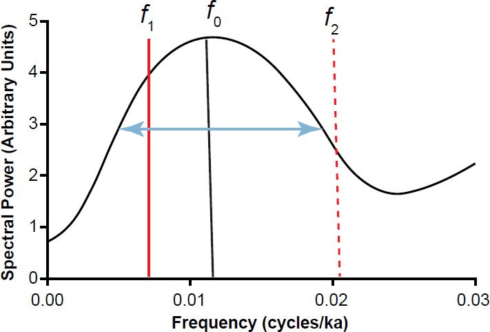
Fig. 7. If a frequency f falls within the full-width at half-maximum (FWHM), indicated by the horizontal blue ray, then it may be considered equal to the frequency f of the peak, within experimental uncertainty. This is not the case for the frequency f , which falls outside the FWHM.
Moreover, the Pacemaker authors pointed out that the ratio of the obliquity to precession periods ought to be about 41÷23=1.78≈1.8. Since the ratio of the B peak period to the C peak period was close to (within 5% of) this value for the RC11-120 and E49-18 SIMPLEX spectra, this was seen as additional evidence for Milankovitch climate forcing (Hays, Imbrie, and Shackleton 1976, 1127). In fact, these ratios were also close to the expected values for the PATCH spectra, as well (see their table 4).
Of course, the peaks must also be statistically distinguishable from the background. The Pacemaker authors acknowledged that this was a necessary (though not necessarily a sufficient) condition for acceptance of Milankovitch theory (Hays, Imbrie, and Shackleton 1976, 1127). Given the great importance of the Pacemaker results, it is not unreasonable to expect that at least some of the spectral peaks would be distinguishable from the background, even for 90% and 95% confidence intervals. Likewise, this should be true, not just for the low frequency A peaks, but also for at least some of the higher frequency B and C peaks.
Procedure
Now I attempt to see if simple age models for the RC11-120 and E49-18 cores might still yield results that are consistent with Milankovitch expectations, after taking into account the new age for the B-M reversal boundary, as well as data from the upper section of the E49-18 core. If simple age models yield results that are consistent with Milankovitch expectations, then I am justified in experimenting with more complex age models, as did the Pacemaker authors.
Interpolation of the original data tends to enhance the power of low frequency spectral components at the expense of power at higher frequencies (Schulz and Mudelsee 2002, 421). Hence, to keep the test as fair as possible, I attempted to keep interpolation to a minimum whenever possible. I did this by choosing time increments Δt for the interpolated data that were close to the time increments for the uninterpolated data. I attempted to determine empirically (by trial and error) values of m that would be most favorable to Milankovitch expectations. I chose a single value of m for all three spectra within a given age model trial. The chosen value of m then determined the bandwidth and the number of degrees of freedom in any potential test of statistical significance. Once the value of m used to obtain the three power spectra was chosen, another single (small) value of m was found (again, by trial and error) that gave the best overall fitting null continua for all three spectra.
I restricted myself to values of m that were all integer multiples of 5, for two reasons: first, to avoid the charge that I chose unusual values of m in an attempt to “rig” the results, and second, to keep the number of test trials (for different potential values of m) manageable.
Since I have already shown that I can replicate fairly well the original Pacemaker results (even in the high-frequency parts of the spectra), I here show only the “interesting” parts of the unprewhitened power spectra, for frequencies less than or equal to 0.08 cycles/ka. However, for the cases in which I prewhitened the data, I plotted the entire frequency range, so that the reader could judge whether my choice of prewhitening constant C did a reasonably good job of “flattening” the spectrum. Since it is permissible when using the Blackman-Tukey method to set the number of frequencies to 2 to 3 times the value of m (Jenkins and Watts 1968, 260), I plotted these spectra at higher resolution (with the number of frequencies set to 3m), which should enable the reader to see more detail in the spectral peaks.
For each (unprewhitened) trial, I used vertical lines to indicate the frequencies/periods corresponding to the obliquity and precession cycles. In the last two trials, which were characterized by relatively long timescales (> 500 ka), I also calculated the eccentricity frequencies/periods and plotted those, as well.
In the following figures, solid red curves indicate null continua, blue brackets indicate bandwidths, and thin green and blue lines (when included) indicate, respectively, the bounds of the 80% and 90% confidence intervals. The numbers in bold indicate my estimates (in ka) for the periods of the dominant spectral peaks. When B and C peaks were both present in a spectrum, I also included both the theoretical and experimentally determined obliquity-to-precession ratios.
An Assumed Age of 127 ka for the MIS 6-5 Boundary: New Results
In an attempt to “dodge” the potential causality problems discussed above, I refrained from using in my first trial any chronological anchor points that were directly tied to the age of the B-M reversal boundary. This leaves the original SIMPLEX results for the RC11-120 core unaffected, as neither of its two anchor points were tied to that boundary. However, prewhitening of the three RC11-120 data sets (Figs. 8–10) using a prewhitening constant of C = 0.70 reveals that none of the B and C peaks are statistically distinguishable from the background. Likewise, examination of Figs. 9–11 in Hebert (2016b) suggests that the low-frequency A peaks are not significant either, as the lower bounds of the 80% confidence intervals for the A peaks fall below the null continua, with the possible exception of the δ18O A peak. However, bias may cause the B-T method to overestimate the significance of low-frequency peaks (Weedon 2003, 85). In that case, none of the A peaks (including the δ18O A peak) are significant, even if one ignores the difficulty of estimating the long eccentricity period from such a short time interval. These results are not surprising, as the n and m values used by the Pacemaker authors imply that the number of degrees of freedom ν for the RC11-120 core was just 6, even if one used the more generous estimate for the number of degrees of freedom, Eq. (41) in Hebert (2016b). Generally, eight degrees of freedom is considered a bare minimum for such a spectral analysis (Weedon 2003, 69, 71). The RC11-120 core is just too short, given our degree of blurring, to obtain statistically significant results.
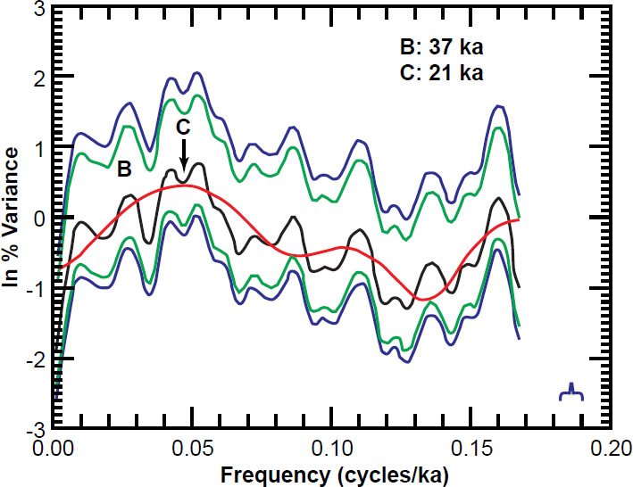
Fig. 8. Prewhitened RC11-120 SST power spectrum (C = 0.70), obtained using the same values of m and n as in the original Pacemaker paper. The null continuum (red curve) was obtained with m = 7. Blue bracket is the bandwidth, and green and blue lines are the bounds of the 80% and 90% confidence intervals, respectively.
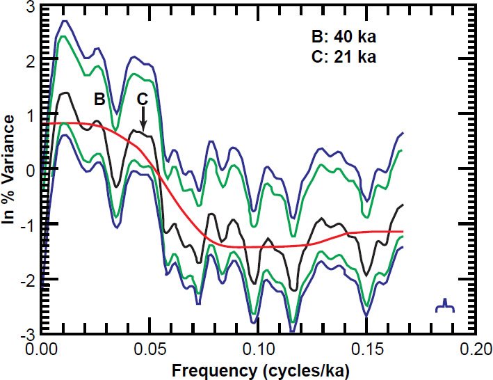
Fig. 9. Prewhitened RC11-120 δ18O power spectrum (C = 0.70), obtained using the same values of m and n as in the original Pacemaker paper. The null continuum (red curve) was obtained with m = 7. Blue bracket is the bandwidth, and green and blue lines are the bounds of the 80% and 90% confidence intervals, respectively.
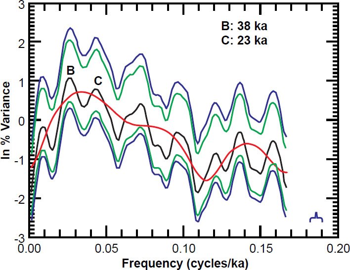
Fig. 10. Prewhitened RC11-120 % C. davisiana power spectrum (C = 0.70), obtained using the same values of m and n as in the original Pacemaker paper. The null continuum (red curve) was obtained with m = 7. Blue bracket is the bandwidth, and green and blue lines are the bounds of the 80% and 90% confidence intervals, respectively.
The only two E49-18 anchor points not tied to the age of the B-M reversal boundary are the age of 127 ka for the MIS 6-5 boundary and, if one is willing to use it, Howard and Prell’s (1992, 87, 91) estimated age of 12 ka for the core top. One may argue that it is unreasonable to perform a spectral analysis on a 15.5m long core using only two anchor points separated by less than a third of this distance. However, if one wishes to “dodge” the potential causality problems discussed above by refraining from using E49-18 anchor points whose ages were tied to the B-M reversal boundary, it’s either these two anchor points, or nothing!
The time increment between uninterpolated data points was 2.347 ka, so I interpolated the data using Δt = 2.35 ka. This resulted in n = 155 data points.
Even if spectral peaks occur at frequencies predicted by the Milankovitch theory, those results will not be convincing unless they are also statistically significant. Because this is the only opportunity to obtain statistically significant results for the SIMPLEX age model while simultaneously “dodging” a potential causality problem, I chose as a starting value the largest possible value of m that would still result in the requisite eight degrees of freedom. Eq. (41) in Hebert (2016b) shows that this can be achieved with m=50 (ν=7.80≈8). The null continua were obtained by setting m=7. If the initial results are in reasonable agreement with Milankovitch expectations, then one can experiment with still smaller values of m (say, m=40) to see if the results will continue to be consistent with Milankovitch expectations for narrower confidence intervals. One drawback of using m=50 for this trial, however, is that the resulting spectral resolution is too coarse to see a clear eccentricity peak at f~0.01 cycles/ka. However, given the relative shortness of this particular timescale (362 ka), this is not really an issue anyway. Hence, I did not calculate a theoretical eccentricity period for this trial.
As one can see from Figs. 11–13, agreement with Milankovitch expectations is very poor. The predicted obliquity frequencies do not fall within the FWHM of any of the B peaks. Nor does the predicted precession frequency fall within the FWHM of the SST C peak. One could perhaps argue that the precession frequencies fall within the FWHM of the δ18O and % C. davisiana C peaks, but these peaks are extremely small anyway, and are arguably not really peaks at all. Note also that the δ18O and % C. davisiana obliquity/precession ratios of ~1.6 and ~1.5 agree poorly with the expected value of ~1.8.
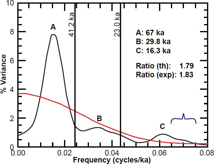
Fig. 11. Unprewhitened SST power spectrum (m = 50) for the entire E49-18 core using the core top (12 ka) and a depth of 4.90 m (127 ka) as chronological anchor points. The null continuum (red curve) was obtained with m = 7. The blue bracket indicates the bandwidth, and vertical lines indicate the obliquity and precession frequencies/ periods for this time interval.
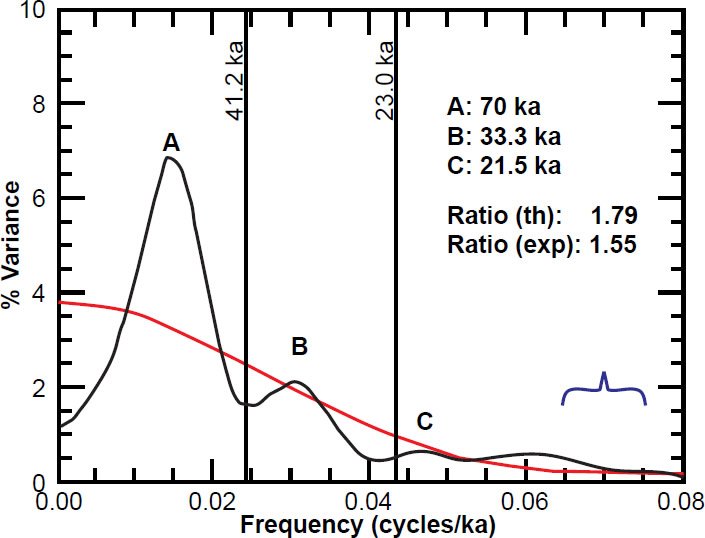
Fig. 12. Unprewhitened δ18O power spectrum (m = 50) for the entire E49-18 core using the core top (12 ka) and a depth of 4.90 m (127 ka) as chronological anchor points. The null continuum (red curve) was obtained with m = 7. The blue bracket indicates the bandwidth, and vertical lines indicate the obliquity and precession frequencies/periods for this time interval.
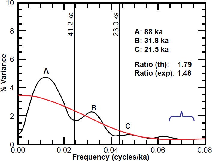
Fig. 13. Unprewhitened % C. davisiana power spectrum (m = 50) for the entire E49-18 core using the core top (12 ka) and a depth of 4.90 m (127 ka) as chronological anchor points. The null continuum (red curve) was obtained with m = 7. The blue bracket indicates the bandwidth, and vertical lines indicate the obliquity and precession frequencies/periods for this time interval.
An Assumed Age of 143 ka for the MIS 6-5 Boundary: New Results
If one does not use the disputed upper section of the E49-18 core, then the only remaining available E49-18 age control points used in the original Pacemaker analysis are the MIS 6-5, 8-7, and 12-11 boundaries. As noted earlier, in the case of the bottom section of the E49-18 core, it is more favorable to the Milankovitch theory to avoid “mixing” the age estimate of 127 ka for the MIS 6-5 boundary with the revised age estimate of 491 ka for the 12-11 boundary. This means that if one intends to refrain from using the disputed upper section of the E49-18 core, then all the age estimates for the MIS boundaries should be obtained from the V28-238 core. In other words, we will use the age estimates of 143, 280, and 491 ka for these three MIS boundaries, despite the potential causality problems involved.
In this trial, I attempted to obtain the results from the RC11-120 and E49-18 cores that were most favorable to the Milankovitch theory, even if those results were not statistically significant, as this was the approach used by the Pacemaker authors. If the RC11-120 and E49-18 B and C spectral peaks are in reasonable agreement with Milankovitch expectations, then one can form a new PATCH “core”, based on the new timescale, and see if the PATCH spectra will then also be consistent with Milankovitch expectations.
Figs. 14–16 show the new SIMPLEX results for the RC11-120 core. These were obtained with n = 96, Δt = 3.25 ka (no interpolation was necessary), and m = 40. The null continua were obtained by setting m = 5. The spectrum has been sufficiently blurred so that the frequencies of the B and C SST and δ18O peaks arguably coincide with the theoretically expected frequencies. However, the degree of blurring means that one can make a case that the width of the δ18O B peak (Fig. 15) is too small relative to the bandwidth to be counted as a separate spectral feature. Note also that the vertical line representing the frequency of the precession cycle is outside the FWHM of the % C. davisiana C peak (Fig. 16). Also the δ18O and % C. davisiana C peaks still fail to meet the criterion in the original Pacemaker paper: these peak frequencies are not within 5% of the theoretical values. In fact, the δ18O and % C. davisiana B peaks also (just barely) fail to meet this requirement, as well. Likewise the δ18O and % C. davisiana obliquity/precession ratios of ~1.6 are significantly smaller than the expected value of ~1.8.
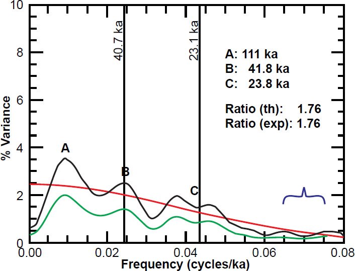
Fig. 14. Unprewhitened RC11-120 SST power spectrum (m = 40), using the original SIMPLEX age model, but with the second chronological anchor point based upon an age of 780 ka, rather than 700 ka, for the B-M magnetic reversal boundary. The null continuum (red curve) was obtained with m = 5. The blue bracket is the bandwidth, and the light green line is the lower bound of the 80% confidence interval. Vertical lines indicate the obliquity and precession frequencies/periods for this time interval.
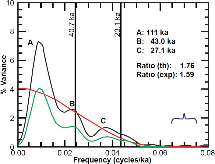
Fig. 15. Unprewhitened RC11-120 δ18O power spectrum (m = 40), using the original SIMPLEX age model, but with the second chronological anchor point based upon an age of 780 ka, rather than 700 ka, for the B-M magnetic reversal boundary. The null continuum (red curve) was obtained with m = 5. The blue bracket is the bandwidth, and the light green line is the lower bound of the 80% confidence interval. Vertical lines indicate the obliquity and precession frequencies/periods for this time interval.
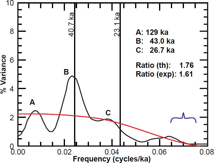
Fig. 16. Unprewhitened RC11-120 % C. davisiana power spectrum (m = 40), using the original SIMPLEX age model, but with the second chronological anchor point based upon an age of 780 ka, rather than 700 ka, for the B-M magnetic reversal boundary. The null continuum (red curve) was obtained with m = 5. The blue bracket is the bandwidth, and vertical lines indicate the obliquity and precession frequencies/periods for this time interval.
Figs. 17–19 show the new SIMPLEX results for the E49-18 core (bottom section only). For the uninterpolated data, Δt varied slightly (due to round-off error) between 3.800 and 3.801 ka. Interpolation was thus performed with Δt=3.8 ka, implying that n=107. The truncation point was chosen to be m=40, and the null continua were obtained by setting m=8. In general, this trial yields much poorer agreement with Milankovitch expectations: with the possible exception of the SST B peak, none of the B and C peaks agree with expectations, according to the FWHM rule (or the 5% rule, for that matter). As in the original Pacemaker paper, the B and C peaks are not present in the % C. davisiana spectrum. However, the SST and δ18O obliquity/precession ratios agree fairly well with the expected values, although they are a little high.
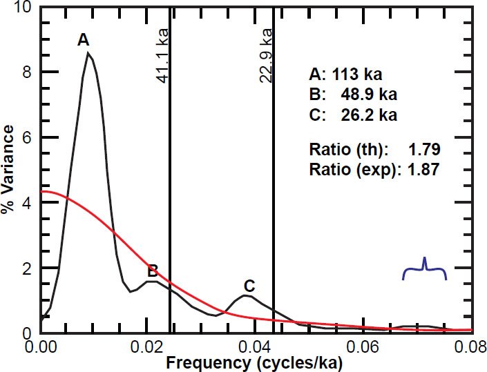
Fig. 17. Unprewhitened SST power spectrum (m = 40) for the bottom of the E49-18 core, using the original SIMPLEX age model, but with age anchor points tied to an age of 780 ka, rather than 700 ka, for the B-M magnetic reversal boundary. The null continuum (red curve) was obtained with m = 8. The blue bracket indicates the bandwidth, and vertical lines indicate the obliquity and precession frequencies/periods for this time interval.
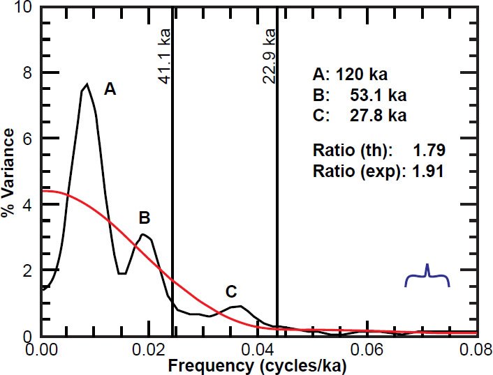
Fig. 18. Unprewhitened δ18O power spectrum (m = 40) for the bottom of the E49-18 core, using the original SIMPLEX age model, but with age anchor points tied to an age of 780 ka, rather than 700 ka, for the B-M magnetic reversal boundary. The null continuum (red curve) was obtained with m = 8. The blue bracket indicates the bandwidth, and vertical lines indicate the obliquity and precession frequencies/periods for this time interval.
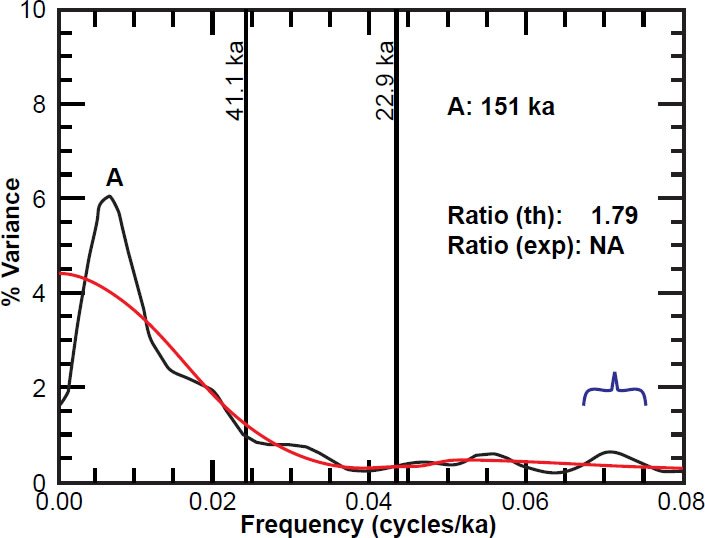
Fig. 19. Unprewhitened % C. davisiana power spectrum (m = 40) for the bottom of the E49-18 core, using the original SIMPLEX age model, but with age anchor points tied to an age of 780 ka, rather than 700 ka, for the B-M magnetic reversal boundary. The null continuum (red curve) was obtained with m = 8. The blue bracket indicates the bandwidth, and vertical lines indicate the obliquity and precession frequencies/periods for this time interval.
Given these equivocal results, one cannot really justify constructing a composite PATCH “core.” However, for the sake of completeness, I did so anyway.
I should now mention still another potential problem with the Pacemaker paper that escaped my notice while writing the first two papers in this series. Our null hypothesis is that the seafloor sediment data are generated by a weakly stationary random process. For a weakly stationary process, the covariance should depend only on the lag, but not on the section of the data for which the covariance is calculated. In other words, for a given lag value, the first half of the data should yield approximately the same covariance as the second half of the data (assuming the data set is reasonably large). Since the variance is just the covariance evaluated for a lag of zero, this implies that the variance should be constant in time. In the case of the PATCH “core,” this means that the variance of the detrended data from the RC11-120 core segment and the variance of the detrended data from the E49-18 core segment should be about the same. This was approximately true for the δ18O and % C. davisiana data. The two variances for the detrended δ18O data segments were 0.17 and 0.13, and the two variances for the detrended % C. davisiana data segments were 16 and 21. However, the variances for the two SST data segments were 2.3 and 6.0. Hence, it seems that the variances of the detrended data segments should have been normalized prior to the analysis by dividing each value in the detrended data segment by the standard deviation for that particular data segment. This would force both data segments to have a variance of one, allowing us to maintain our assumed condition of weak stationarity. Based on the good agreement between my PATCH results and those presented in the original Pacemaker paper, it is not clear that the authors did this. Nor did I do it when producing this paper’s Figs. 2–4 and Figs. 15–17 in Hebert (2016b). However, this did not make much of a difference in the final results, even for the SST PATCH power spectrum (Fig. 20). However, for the sake of rigor in the following calculations, I normalized the variances for each detrended data segment before combining them into a composite PATCH data set.
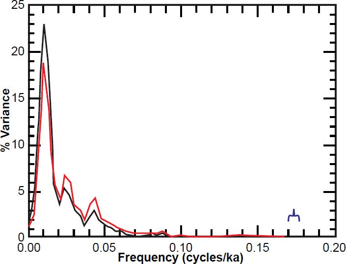
Fig. 20. Unprewhitened SST PATCH power spectrum (m = 50) based upon an assumed age of 700 ka for the B-M magnetic reversal boundary, for the cases when the variances of the two detrended data sets used to construct the PATCH “core” were normalized (red curve) and not normalized (black curve) The blue bracket indicates bandwidth.
All age control points were left unchanged from the original Pacemaker paper except those that were tied to the age of the B-M reversal boundary. In the new uninterpolated PATCH timescale, Δt ranged from a minimum of 2.41 ka to a maximum of 3.96 ka, but nearly all the time increments were between 3.33 ka and 3.96 ka. The average time increment was very close to 3.6 ka, so I set Δt = 3.6 ka, resulting in n = 152. Since this is the last opportunity to obtain a significant result within this particular trial, one would prefer to set m=50, which would result in the minimum requisite eight degrees of freedom (Weedon 2003, 69, 71). However, given the length of this trial’s time interval (544 ka), one can reasonably calculate an eccentricity period. But this requires a larger value of m in order to discern a clear spectral peak at ~0.01 cycles/ka. Hence, these results were obtained with m=65. The null continua were obtained with m=7.
These results are depicted in Figs. 21–23. Agreement with the Milankovitch theory is again generally poor, especially for the B and C peaks. None of the B or C peak frequencies agreed with predicted values, either by the Pacemaker authors’ 5% rule or by the FWHM rule. However, the calculated obliquity/precession ratios are in good agreement with the expected value of ~1.8. One could attempt to argue that the small D peak in the δ18O spectrum is a precession peak, which would mean that the frequency of the D peak is in agreement with Milankovitch expectations. However, this would raise the B-C period ratio to 2.16, in extremely poor agreement with the expected ratio of 1.75.
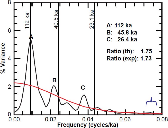
Fig. 21. Unprewhitened SST PATCH power spectrum (m = 65), using the original ELBOW age model, but with age anchor points tied to an age of 780 ka, rather than 700 ka, for the B-M magnetic reversal boundary. The null continuum (red curve) was obtained with m = 7. The blue bracket indicates the bandwidth, and vertical lines indicate the eccentricity, obliquity, and precession frequencies/periods for this time interval.
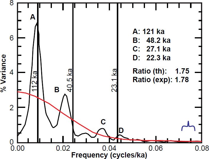
Fig. 22. Unprewhitened δ18O PATCH power spectrum (m = 65), using the original ELBOW age model, but with age anchor points tied to an age of 780 ka, rather than 700 ka, for the B-M magnetic reversal boundary. The null continuum (red curve) was obtained with m = 7. The blue bracket indicates the bandwidth, and vertical lines indicate the eccentricity, obliquity, and precession frequencies/periods for this time interval.
Fig. 23. Unprewhitened % C. davisiana PATCH power spectrum (m = 65), using the original ELBOW age model, but with age anchor points tied to an age of 780 ka, rather than 700 ka, for the B-M magnetic reversal boundary. The null continuum (red curve) was obtained with m = 7. The blue bracket indicates the bandwidth, and vertical lines indicate the eccentricity, obliquity, and precession frequencies/periods for this time interval.
In the last trial, I used data from the entire E49-18 core, along with anchor points that were tied to the B-M reversal boundary. Of course, this resulted in the “causality” issues discussed above, but at this point, this cannot be helped, as this is essentially the last remaining opportunity to confirm the Milankovitch theory using these core data. Given the length of the E49-18 core, it seems only fair to use three chronological anchor points to construct the timescale, as changes in sedimentation rate are more likely in a long core such as this one. Thus, I used the core top (assumed age of 12 ka), the MIS 8-7 boundary (assumed age of 280 ka), and the MIS 12-11 boundary (assumed age of 491 ka). In the original Pacemaker paper, the MIS 6-5 boundary was arguably a more important control point than the MIS 8-7 boundary, due to the fact that its age had “been the cornerstone of some previous attempts to support specific versions of the orbital hypothesis” (Hays, Imbrie, and Shackleton 1976, 1124). Moreover, the original age estimate of 127–128 ka for this boundary was in reasonable agreement with Milankovitch expectations. However, now that the revised age for the B-M reversal boundary has changed this age estimate to 143 ka, there seems to be no reason to favor this particular age control point over the MIS 8-7 boundary. Since the MIS 8-7 boundary is roughly halfway down the length of the E49-18 core, it seems to be a fairer, more logical choice for the second age control point. These anchor points implied time increments between data points of 3.24 and 3.64 ka, so I set Δt=3.44 ka as a compromise value, which implied a value of n=155. One would prefer to set m=50, so that there would be the requisite eight degrees of freedom (Weedon 2003, 69, 71), since this is the last opportunity for statistically significant results. However, the length of this trial’s time interval (530 ka) necessitates an estimate for the eccentricity period, which requires a larger value of m. Hence, these results were obtained with m=60, and the null continua were obtained with m=8.
The results are shown in Figs. 24–26. The precession spectrum actually yielded two peaks, a large peak corresponding to 23 ka and a much smaller peak corresponding to 19 ka. Because the second of these peaks is much smaller than the first, I have only included the 23.0 ka precessional frequency/ period on the figures. With the possible exception of the δ18O C peak, the SST and δ18O B and C peaks do not agree with Milankovitch expectations. However, the % C. davisiana B and C peaks arguably agree with expectations by the FWHM rule, and the % C. davisiana C peak also agrees by the 5% rule. Note also that the obliquity/precession ratios of ~2.0, 2.3, and ~2.0 are in poor agreement with the expected value of ~1.8.
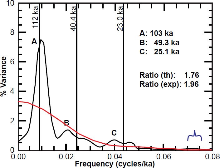
Fig. 24. Unprewhitened SST spectrum for the entire E49-18 core (m = 60) using a simple age model implied by an age of 780 ka, rather than 700 ka, for the B-M magnetic reversal boundary. The age control points were the core top (12 ka), 8.25 m (280 ka), and 14.05 m (491 ka). The null continuum (red curve) was obtained with m = 8. The blue bracket indicates the bandwidth, and vertical lines indicate the eccentricity, obliquity, and precession frequencies/periods for this time interval.
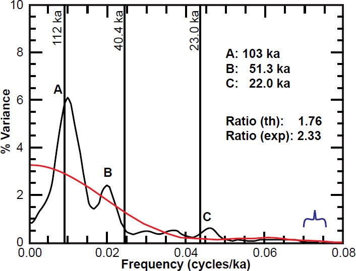
Fig. 25. Unprewhitened δ18O spectrum for the entire E49-18 core (m = 60) using a simple age model implied by an age of 780 ka, rather than 700 ka, for the B-M magnetic reversal boundary. The age control points were the core top (12 ka), 8.25 m (280 ka), and 14.05 m (491 ka). The null continuum (red curve) was obtained with m = 8. The blue bracket indicates the bandwidth, and vertical lines indicate the eccentricity, obliquity, and precession frequencies/periods for this time interval.
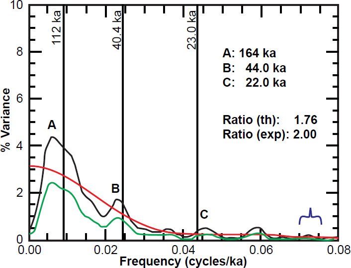
Fig. 26. Unprewhitened % C. davisiana spectrum for the entire E49-18 core (m = 60) using a simple age model implied by an age of 780 ka, rather than 700 ka, for the B-M magnetic reversal boundary. The age control points were the core top (12 ka), 8.25 m (280 ka), and 14.05 m (491 ka). The null continuum (red curve) was obtained with m = 8. The blue bracket indicates the bandwidth, and vertical lines indicate the eccentricity, obliquity, and precession frequencies/periods for this time interval. The green line indicates the lower bound of the 80% confidence interval.
In summary, when the new age of the B-M magnetic reversal is taken into account, none of these trials provide convincing evidence for the Milankovitch theory, regardless of whether or not one includes in the analysis the disputed uppermost data from the E49-18 core. This is especially true if one considers the potential causality problems implied by an age of 780 ka for the B-M magnetic reversal boundary. Of course, Milankovitch proponents may try to argue that there are other convincing arguments for Milankovitch climate forcing, a possibility we discuss later in this paper.
Implications for the “Climate Change” Debate
These results have important implications for the debate over “global warming” or “climate change.” As noted by (Vardiman 2001, 79), the fact that Milankovitch-induced variations in the distribution of solar insolation appear insufficient, in and of themselves, to account for presumed past climate change, has forced uniformitarian paleoclimatologists to postulate secondary “feedback mechanisms” to amplify these effects:
A major result of this need for feedback mechanisms has been the development of a perspective that the earth’s climate system is extremely sensitive to minor disturbances. A relatively minor perturbation could initiate a non-linear response which might lead to another “Ice Age” or “Greenhouse.” Because of the fear that a small perturbation might lead to serious consequences, radical environmental policies on the release of smoke, chemicals, and other pollutants and the cutting of trees have been imposed by international agencies and some countries. If the basis for the Astronomical Theory is wrong, many of the more radical environmental efforts may be unjustified.
A survey of the uniformitarian literature reveals a plethora of papers which infer, based on Milankovitch/ uniformitarian interpretations of paleoclimatological data, that our climate is unstable: see, for example Alley et al. (1997), Dansgaard et al. (1993), Greenop et al. (2014), Keeling and Stephens (2001), Sandal and Nof (2008), Schilman et al. (2001), and Thompson et al. (1997).
In this light, it is worth noting that many in Christendom have concluded that combatting “climate change” is a moral imperative, including Pope Francis and a number of evangelical leaders (see for instance, the document Climate Change: An Evangelical Call to Action archived, as of 1/6/2016, at http://www.npr.org/documents/2006/feb/evangelical/calltoaction.pdf). Do they realize that much of the alarmism over this issue is stemming from an implicit denial of biblical history?
Implications for Uniformitarian Geochronology
The Pacemaker paper is the basis for acceptance of the modern version of the Milankovitch theory, which plays an extremely important role in geochronology, as it is used to assign ages to other seafloor sediment cores via a technique known as “orbital tuning” (Herbert 2010). These presumed ages for the seafloor sediments are then used to assign ages to other seafloor sediments (Pahnke et al. 2003), as well as to the deep ice cores of Greenland and Antarctica (Waelbroeck et al. 1995). Finally, some of these ice cores are then used to assist in the dating of other seafloor sediment cores (Pahnke et al. 2003). The Milankovitch hypothesis is even used to calibrate Ar-Ar radioisotope dating standards (Channell et al. 2010; Huang, Hesselbo, and Hinnov 2010; Meyers et al. 2012; Renne et al. 1994; Rivera et al. 2011)!
Ages assigned to a particular ice or sediment core are often “tied” to multiple other cores. Both a technical (Hebert 2015) and a popular level article (Hebert 2016c) describe how the age assignments for the MD97-2120 sediment core off the coast of New Zealand were “tied” to other deep-sea sediment and ice cores (Fig. 27).
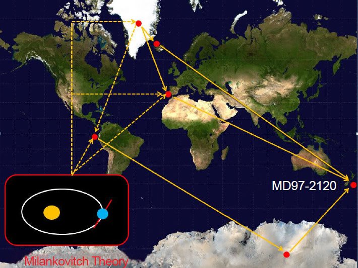
Fig. 27. Age assignments for marine sediment cores, such as the New Zealand MD97-2120 core, are often tied to age assignments for other sediment and ice cores, and these ages are usually tied to Milankovitch expectations. Image credit for Mercator map projection: Wikimedia Commons, public domain. https://commons.wikimedia.org/wiki/File:Mercator-projection.jpg.
But in the absence of clear evidence for its validity, use of the Milankovitch hypothesis to help construct a secular geochronology amounts to no more than a gigantic exercise in circular reasoning, as discussed in (Hebert 2014, 2015, 2016a). Neeman (1993) has demonstrated that it is possible for randomly generated computer signals—having no connection whatsoever to real-world climate—to be convincingly “tuned” to Milankovitch expectations! Others have also expressed concerns about the dangers inherent in orbital tuning (Blaauw 2010; Blaauw, Bennett, and Christen 2010). This is why the Pacemaker paper is so important: it supposedly provided the logical rationale for the orbital tuning technique.
There are likely hundreds, if not thousands, of published papers that assume the validity of Milankovitch forcing and then use that assumption to help construct an “old-earth” geochronology. Without a firm basis for this assumption, the conclusions of all those papers are automatically suspect, even by uniformitarian reckoning.
Why the Age Revision for the B-M Reversal Boundary?
The Brunhes-Matuyama magnetic reversal has undergone significant revisions over the years. In 1968, its age was estimated to be between one million and 700,000 years (Doell et al. 1968). In 1969, the age assignment, based upon K-Ar dating, was 690 ka (Broecker and Van Donk 1970, 180; Cox 1969, 240). By 1973, the accepted age was 700 ka (Shackleton and Opdyke 1973, 40). Sometime prior to 1979, it was adjusted upward slightly to 710 ka (Mankinen and Dalrymple 1979, 623). In 1979, the age (based on a large study using newly revised K-Ar dating constants) was revised to 730±11 ka (Imbrie et al. 1984, 285; Mankinen and Dalrymple 1979, 623). As noted by Muller and MacDonald (2000, 153), this age for the B-M reversal boundary was then seemingly confirmed by a number of astronomical tuning studies (Kominz et al. 1979; Kominz and Pisias 1979; Morley and Hays 1981). However, there was a notable outlier: Johnson (1982) had obtained an age estimate of 790±5 ka via marine-astronomical correlations.
In passing, there is a certain historical irony in Johnson’s result. Hays, Imbrie, and Shackleton (1976) used an assumed age of 700 ka for the B-M magnetic reversal boundary to confirm the validity of Milankovitch climate forcing. But Johnson then assumed the validity of Milankovitch climate forcing, and then “proved” that the age of the B-M reversal boundary was really 790 ka!
In the early 1990s Shackleton, Berger, and Peltier (1990) developed an astronomically tuned timescale for the ODP 677 core, located off the Galapagos Islands. As they noted (their p.258), their revised timescale “requires ages for the last few reversals of the earth’s magnetic field that are around 5–7% greater than the currently accepted values.” As the age of the Brunhes-Matuyama magnetic reversal was then believed to be 730 ka, this implied an upward revision to 780 ka (their Table 4, p.257).
Likewise, other scientists (Hilgen 1991) were making a similar argument based upon other sediment cores from the Mediterranean. Herbert (2010, 374) describes how a Dutch team of researchers also concluded that the ages for the most recent reversal boundaries should be revised upward:
Hilgen and co-workers recognized orbital forcing [in Mediterranean sediment cores] by a grouping of sapropels (dark, organic-rich beds) into units of ~100 and 400ky by eccentricity modulation of precessional climate changes. Their resulting calibration of the GPTS [geomagnetic polarity timescale] yielded significantly greater ages for magnetic reversal boundaries than the previously accepted ages based on K/Ar radiometric age dating. After initial controversy, the ages proposed by Hilgen and others have largely been verified by recent advances in 40Ar/39Ar dating of volcanic ash layers at a number of magnetic reversal boundaries.
Hence, secular scientists used a presumed age of 700 ka for the B-M magnetic reversal boundary to convince the world of the validity of Milankovitch climate forcing. But this age estimate was revised upward, with the final revision to 780 ka resulting from an attempt to “tune” the chemical wiggles within other sediment cores (Fig. 28) into alignment with Milankovitch expectations!
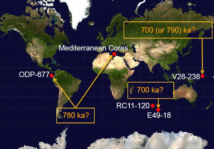
Fig. 28. Uniformitarian scientists used the E49-18 and V28-238 sediment cores and an assumed age of 700 ka for the Brunhes-Matuyama magnetic reversal to convince the scientific community of the reality of Milankovitch climate forcing. However, in order to tune chemical wiggles within core ODP-677 and multiple Mediterranean cores into alignment with Milankovitch expectations, they had to revise the age of the B-M reversal boundary to 780 ka. Likewise, Johnson (1982) argued that the age of the B-M reversal boundary was really 790 ka. Image credit for Mercator map projection: Wikimedia Commons, public domain. https://commons.wikimedia.org/wiki/File:Mercator-projection.jpg.
Tauxe et al. (1992) claimed that, when uncertainties were properly taken into account, the 95% confidence interval for the age of the B-M magnetic reversal boundary extended from 730 to 780 ka. However, even this generous error estimate does not reconcile the contradiction between these age assignments and the earlier age estimate of 700 ka that was actually used to obtain the Pacemaker results.
Had Hilgen and Shackleton et al. not “needed” a higher age for the B-M reversal boundary, it is likely that Johnson’s anomalously high age estimate of 790 ka would have quickly been forgotten. Indeed, Imbrie et al. (1984, 301) argued against it on the basis of orbital tuning results. But because uniformitarian paleoclimatologists had difficulty tuning the “wiggles” in other sediment cores to Milankovitch expectations without the higher age estimate, uniformitarian paleoclimatologists quickly adopted it, and it was then “confirmed” by radioisotope dating (Baksi et al. 1992; Spell and McDougall 1992; Tauxe et al. 1992).
Herbert (2010, 374) points out that this revision was accompanied by “initial controversy”. It’s not hard to see why. First, K-Ar dating experts would have been understandably irritated that paleoclimatologists simply overruled their age estimates. Yes, the revised age of 780–790 ka was supposedly confirmed by radioisotope dating after the fact, but at the time the revision was proposed, there seems to have been little, if any, real justification, for a higher age for the B-M reversal boundary. Remember that the estimates of Johnson, Hilgen, and Shackleton et al. were all based upon astronomical, rather than radioisotopic, considerations. Rather than simply allowing the Milankovitch theory to be falsified, uniformitarian scientists raised the age of the B-M reversal boundary, disregarding their own earlier radioisotope dating estimates. Only after the higher age was “needed” by the Milankovitch theory did the radioisotope justification ostensibly follow. Why does one get the feeling that the Milankovitch theory is leading radioisotope dating methods around by the nose? Is this just another example of the “reinforcement syndrome” in science, in which results are (perhaps unconsciously) “massaged” to agree with the supposed “correct” value (Oard 2013)?
Second, scientists who were aware that the Pacemaker results were tied to a much lower age estimate (700 ka) for the B-M reversal boundary would have realized that this revision had the potential to logically undermine both the evidence for the Milankovitch theory and the concept of orbital tuning. Hence it is easy to see why such a revision would have been—and indeed, should have been— controversial at the time.
Nevertheless, uniformitarian scientists consider the currently accepted age estimate of 780 ka for the B-M reversal boundary to be a great triumph for the orbital tuning process (Berger 2014, 169; Muller and MacDonald 2000, 156). It looks to me like circular reasoning, but even if we accept, for the sake of argument, this new age estimate, we have already seen that it introduces very serious problems into the original Pacemaker analysis.
But Isn’t There Other Evidence for the Milankovitch Theory?
Milankovitch proponents will likely claim that there are other strong arguments for Milankovitch climate forcing. After all, there are hundreds, if not thousands, of published papers involving the Milankovitch theory. True, but most of them simply assume that the theory is correct and use that assumption to orbitally “tune” chemical wiggles in sediment and ice cores. But how many of these papers provide objective, independent evidence that the theory is actually correct?
Indeed, there are hundreds, if not thousands, of deep seafloor sediment cores in existence. But despite this abundance of cores, providing an objective argument for Milankovitch climate forcing is not a trivial matter. First, one must find a core or cores that are sufficiently long to make a statistically significant case that the chemical “wiggles” are behaving in accordance with the theory (this is the main reason that the original results from the RC11-120 core and the bottom section of the E49-18 core were, by themselves, not convincing evidence for the theory). Second, the core or cores must be reasonably undisturbed. Third, another core, one which records the B-M reversal boundary and is characterized by a very uniform sedimentation rate, is needed to assign age estimates to sediments that are too deep to be tied to radiocarbon or Pa–Th dating methods (remember that the method used to assign ages to the sediments must be independent of Milankovitch assumptions). Finally, these cores must be located in a part of the world where sediment chemical data presumably provides optimal information about past climates. Although several hundred sediment cores had already been studied at the time that the Pacemaker paper was published, the Pacemaker authors claimed that the RC11-120 and E49-18 cores were the only two cores known to them having the right properties for such an analysis (Hays, Imbrie, and Shackleton 1976, 1122). So just because many other cores have been drilled, it does not automatically follow that uniformitarian scientists have performed other tests of the theory.
A reason to suspect that additional objective evidence for the theory is either weak or non-existent is that uniformitarian scientists still greatly emphasize the Pacemaker paper and its importance. If another strong argument for Milankovitch climate forcing did indeed exist, one suspects that uniformitarian paleoclimatologists would emphasize it more.
Finally, a statement by a prominent uniformitarian oceanographer and geologist (Berger 2014, 169) raises a question about the real strength of the evidence for Milankovitch climate forcing. In context, Wolfgang Berger was discussing how earlier timescales for the sediment cores, proposed by scientists such as Cesare Emiliani, had turned out to be wrong:
In the end, the correct timescale [for the marine sediment cores] was a matter of co-ordinating isotope stratigraphy with the results from palaeomagnetism, applying the date found in basalt layers for the Matuyama-Brunhes boundary to cores with known magnetic stratigraphy (as in Shackleton and Opdyke 1973). The agreement of dating by that method and by Milankovitch tuning (urged by Shackleton et al. 1990) is the strongest argument yet for the correctness of Milankovitch theory. (emphasis added)
In light of our discussion so far, Berger’s statement is simply shocking. In order to obtain estimates for the ages of the MIS boundaries that were in reasonable agreement with Milankovitch expectations, Shackleton and Opdyke (1973) used a low estimate (700 ka) for the age of the B-M magnetic reversal boundary. But in order to get “wiggles” in other sediment cores to agree with Milankovitch expectations, Shackleton, Berger, and Peltier (1990) and Hilgen (1991) urged that the age of the B-M reversal boundary be revised upward to 780 ka. How can agreement between these two methods be a “strong” argument for Milankovitch climate forcing when one method requires an age of 700 ka for the B-M magnetic reversal boundary, and the other method requires a completely different age of 780 ka for that same boundary?
Obviously, both ages can’t be right. Are we then supposed to believe that Shackleton and Opdyke simply got “lucky” and obtained age estimates for the MIS boundaries that were approximately correct, even though they used an age for the B-M reversal boundary that was eighty thousand years too young? If Berger is right and this really is the strongest argument yet for Milankovitch climate forcing, then the Milankovitch theory is in serious trouble!
Furthermore, the very fact that uniformitarian paleoclimatologists felt the need to revise upward the age of the B-M reversal boundary is a tacit admission that they have had difficulty reconciling all the data from the different seafloor sediment cores with Milankovitch expectations. Apparently, they can reconcile some of the data with those expectations, but not all of them.
A “More Excellent Way”
Creation scientists do not want to simply criticize uniformitarian thinking. Rather, we want to provide a better alternative. Given these serious problems with the Milankovitch hypothesis, is it perhaps time to try something else?
Creation scientists have long pointed out that there is convincing geological evidence for only one Ice Age in the recent past (Oard 1990, 135–166). The main argument for multiple Pleistocene ice ages is coming, not from glacial deposits themselves, but from uniformitarian interpretations of chemical wiggles in the seafloor sediments. But as this series of papers has demonstrated, this interpretation of the seafloor sediment data is extremely shaky.
Are there clues within the seafloor sediments themselves that would give us hints about past sedimentation rates, clues which do not depend simply on circular reasoning and dubious assumptions?
Yes. Patrick (2010) has noted that the relative scarcity of manganese nodules within the deepest seafloor sediments is a strong argument that the bulk of the seafloor sediments was deposited very rapidly, rather than slowly over millions of years. Since such nodules can only grow at or near the sediment/water interface (Glasby 1978; Pattan and Parthiban 2007), their scarcity in the deepest sediments would imply that nascent manganese nodules lay exposed at this interface only very briefly before being covered by rapidly accumulating sediments. The increasing abundance and size of these nodules at shallower sediment depths is consistent with a gradually decreasing sedimentation rate in the years after the Flood (Fig. 29), as suggested by Vardiman (1996). Such rapid deposition from both continental and biogenic sources would be expected if the year-long Flood described in Genesis is a true historical event. Massive amounts of sheet erosion in the second half of the Flood as the floodwaters drained off the continents would “dump” enormous quantities of sediment into the ocean basins. The rapidly moving water would plane flat large areas on the continents, resulting in numerous “planation surfaces” on every continent (Oard 2011), features which are not currently being formed and which are difficult for uniformitarian scientists to explain (Twidale 1982). Likewise, volcanic activity and rapid seafloor spreading during the Flood event (Baumgardner 1990, 1994a, 1994b, 2003) would have significantly warmed the post-Flood oceans. These warm, mineral-rich waters would have been particularly conducive to the growth of zooplankton, resulting in many so-called “algal blooms.” Since foraminifera and diatoms feed on phytoplankton, they also would likely have greatly proliferated after the Flood, and their remains would have also contributed to the accumulating ocean sediments (Vardiman 1997).
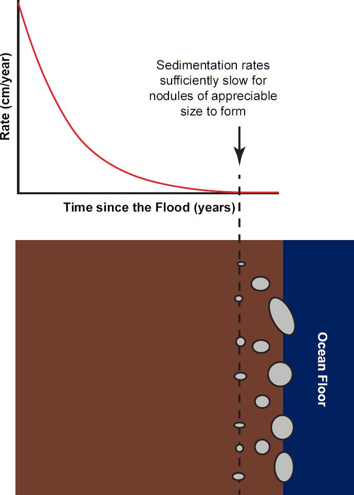
Fig. 29. The general scarcity of manganese nodules within all but the uppermost seafloor sediments can be explained by much higher sedimentation rates at the end of the Genesis Flood and shortly thereafter.
Of course, if rapid seafloor spreading did in fact occur during the Genesis Flood, as believed by most creation scientists, then this would imply that the magnetic reversals recorded in oceanic volcanic rocks occurred very rapidly. Indeed, secular scientists have themselves found strong evidence (Coe and Prévot 1989; Coe, Prévot, and Camps 1995) that a past magnetic reversal occurred in just a little over two weeks, a result that is completely contrary to uniformitarian expectations. Coe has recently repudiated the results (Coe et al. 2014), but this may be due more to “political” pressure (creation scientists had made much of the evidence for these rapid reversals over the years) than a genuine flaw in the initial analysis. Likewise, other uniformitarian scientists (Sagnotti et al. 2014) have also recently argued for rapid changes in the earth’s magnetic field. Furthermore, a respected creation physicist (Humphreys 1990) has proposed a theory to explain these rapid magnetic reversals, a theory which can potentially tie rapid magnetic reversals to the rapid subduction of plates into the earth’s mantle demanded by rapid seafloor spreading during the Flood event.
Furthermore, the warm post-Flood oceans, coupled with residual post-Flood volcanic activity, would have provided ideal conditions for an Ice Age (Oard 1990). Warm oceans would have resulted in dramatically increased evaporation, with increased rain and snowfall. Stratospheric aerosols resulting from residual volcanic activity would provide the necessary summer cooling to allow the growth of thick high-latitude ice sheets. Furthermore, the creation Ice Age model can explain a number of puzzling phenomena (Oard 2005, 35): (a) the existence of pluvial lakes in semi-arid regions during the Ice Age, (b) the apparent “disharmonious” coexistence of warm-climate and cold-climate animals, (c) the lack of glaciation in the Siberian and Alaskan lowlands, and (d) the abundant numbers of woolly mammoths that lived previously in Siberia and Alaska, as well as their eventual extinction.
It should also be noted that there are billions of plant and animal fossils (both terrestrial and marine) preserved in water-deposited sedimentary rocks all over the earth’s surface (Snelling 2009). This is exactly what one would expect from the cataclysmic global Flood described in the Bible.
The Genesis Flood does a much better job of explaining the preponderance of the historical and geological evidence than do uniformitarian assumptions. Of course, there are still unanswered questions. Large amounts of heat are needed to significantly warm the oceans in the Creation/Flood model, but too much heat is definitely a problem: how would excess heat generated by all the geological work done during the Flood be safely dissipated? Although creation scientists have some ideas (Humphreys 2000), we do not yet have a definitive answer to this question. However, uniformitarian scientists have the opposite problem: even if one ignores the problems in the Pacemaker paper that we have just discussed, the changes in summer solar insolation resulting from Milankovitch cycles are much too small in and of themselves to be a convincing explanation for supposed past ice ages. Better to have a potent Ice Age explanation (as is provided by the Creation/Flood model) that can be “dialed back” if need be than to have an explanation (Milankovitch forcing) that is too weak to accomplish the task.
Is a Retraction in Order?
Finally, we return to the question posed in this series’ title: should the Pacemaker paper be retracted? I have not attempted to reproduce the time domain results from the Pacemaker paper, but given the problems already found within the frequency domain analysis, doing so seems unnecessary and would likely constitute “overkill.”
The new age estimate of 780 ka for the B-M magnetic reversal boundary invalidates most of the original results in the frequency domain, including the original test for statistical significance. The SIMPLEX results from the RC11-120 core can still be salvaged, if one assumes that the age of 127 ka for the MIS 6-5 boundary is correct, but these results are, according to my calculations, not statistically significant (without access to the original data it’s impossible to be absolutely sure). Since the Pacemaker authors themselves noted that statistical significance of the predicted spectral peaks is a necessary (but not a sufficient) standard of proof for Milankovitch climate forcing (Hays, Imbrie, and Shackleton 1976, 1127), the Pacemaker paper would seem, by their own reckoning, to no longer provide convincing evidence for Milankovitch climate forcing.
Uniformitarian scientists will no doubt be reluctant to abandon this iconic argument for Milankovitch-induced climate change, but they should, at a minimum, publicly acknowledge to both the larger scientific community and the general public (not to mention government policy makers!) that the Pacemaker results are much weaker than originally presented.
In closing, it is worthwhile to consider some wise counsel from two uniformitarian scientists. Muller and MacDonald (2000, 78) have noted the importance of going back and re-examining old data. They made the following comment in the process of pointing out that a fourth peak (of period 19 ka) “discovered” in the Pacemaker paper was probably not statistically significant:
Is it worthwhile to reanalyse old data? Yes, it is necessary, if we are truly to look at all the data as if for the first time. To untangle the mechanisms of the ice ages, it is very important to know where signals appear, and where they don’t. . . . To solve a jigsaw puzzle, it is just as important to remove pieces that were improperly placed as it is to put new pieces in their correct locations.
Creation scientists could not agree more.
References
Alley, R. B., P. A. Mayewski, T. Sowers, M. Stuiver, K. C. Taylor, and P. U. Clark. 1997. “Holocene Climate Instability: A Prominent, Widespread Event 8200 Yr Ago.” Geology 25 (6): 483–486.
Baksi, A. K., V. Hsu, M. O. McWilliams, and E. Farrar. 1992. “40Ar/39Ar Dating of the Brunhes-Matuyama Geomagnetic Field Reversal.” Science 256 (5055): 356–357.
Baumgardner, J. R. 1990. “3-D Finite Element Simulation of the Global Tectonic Changes Accompanying Noah’s Flood.” In Proceedings of the Second International Conference on Creationism. Vol. 2. Edited by R.E. Walsh and C.L. Brooks, 35–45. Pittsburgh, Pennsylvania: Creation Science Fellowship.
Baumgardner, J. R. 1994a.”Computer Modeling of the Large-Scale Tectonics Associated with the Genesis Flood.” In Proceedings of the Third International Conference on Creationism. Edited by R. E. Walsh, 49–62. Pittsburgh, Pennsylvania: Creation Science Fellowship.
Baumgardner, J. R. 1994b. “Runaway Subduction as the Driving Mechanism for the Genesis Flood.” In Proceedings of the Third International Conference on Creationism. Edited by R. E. Walsh, 63–75. Pittsburgh, Pennsylvania: Creation Science Fellowship.
Baumgardner, J. R. 2003. “Catastrophic Plate Tectonics: The Physics Behind the Genesis Flood.” In Proceedings of the Fifth International Conference on Creationism. Edited by R. L. Ivey Jr., 113–126. Pittsburgh, Pennsylvania: Creation Science Fellowship.
Berger, A. 1978. “Long-Term Variations of Daily Insolation and Quaternary Climatic Changes.” Journal of the Atmospheric Sciences 35 (12): 2362–2367.
Berger, A., and M. F. Loutre. 1991. “Insolation Values for the Climate of the Last 10 Million Years.” Quaternary Science Reviews 10 (4): 297–317.
Berger, W. H. 2014. On the Beginnings of Palaeoceanography: Foraminifera, Pioneers, and the Albatross Expedition. In Landmarks in Foraminiferal Micropalaeontology: History and Development. Edited by A. J. Bowden, F. J. Gregory, and A. S. Henderson, 159–180. London, United Kingdom: Geological Society Publishing House.
Berger, W. H., T. Bickert, G. Wefer, and M. K. Yasuda. 1995. “Brunhes-Matuyama Boundary: 790k.y. Date Consistent with ODP Leg 130 Oxygen Isotope Records Based on Fit to Milankovitch Template.” Geophysical Research Letters 22 (12): 1525–1528.
Blaauw, M. 2010. “Out of Tune: The Dangers of Aligning Proxy Archives.” Quaternary Science Reviews 36: 38–49.
Blaauw, M., K. D. Bennett, and J. A. Christen. 2010. “Random Walk Simulations of Fossil Proxy Data.” The Holocene 20 (4): 645–649.
Blackman, R. B., and J. W. Tukey. 1958. The Measurement of Power Spectra from the Point of View of Communications Engineering. New York: Dover Publications.
Broecker, W. S., and J. van Donk. 1970. “Insolation Changes, Ice Volumes, and the O18 Record in Deep-Sea Cores.” Reviews of Geophysics and Space Physics 8 (1): 169–198.
Channell, J. E. T., D. A. Hodell, B. S. Singer, and C. Xuan. 2010. “Reconciling Astrochronological and 40Ar/39Ar Ages for the Matuyama-Brunhes Boundary and Late Matuyama Chron.” Geochemistry, Geophysics, Geosystems 11 (12): 1–21.
Coe, R. S., and M. Prévot. 1989. “Evidence Suggesting Extremely Rapid Field Variation During a Geomagnetic Reversal.” Earth and Planetary Science Letters 92 (3–4): 292–298.
Coe, R. S., M. Prévot, and P. Camps. 1995. “New Evidence for Extraordinarily Rapid Change of the Geomagnetic Field During a Reversal.” Nature 374 (6524): 687–692.
Coe, R. S., N. A. Jarboe, M. Le Goff, and N. Petersen. 2014. “Demise of the Rapid-Field-Change Hypothesis at Steens Mountain: The Crucial Role of Continuous Thermal Demagnetization.” Earth and Planetary Science Letters 400: 302–312.
Cox, A. 1969. “Geomagnetic Reversals.” Science 163 (3864): 237–245.
Cronin, T. M. 2010. Paleoclimates: Understanding Climate Change Past and Present. New York: Columbia University Press.
Dansgaard, W., S. J. Johnsen, H. B. Clausen, D. Dahl-Jensen, N. S. Gundestrup, C. U. Hammer, C. S. Hvldberg, J. P. Steffensen, A. E. Sveinbjörnsdottir, J. Jouzel, and G. Bond. 1993. “Evidence for General Instability of Past Climate from a 250-Kyr Ice-Core Record.” Nature 364 (6434): 218–220.
Doell, R. R., G. B. Dalrymple, R. L. Smith, and R. A. Bailey. 1968. “Paleomagnetism, Potassium-Argon Ages, and Geology of Rhyolites and Associated Rocks of the Valles Caldera, New Mexico.” Geological Society of America Memoirs 116: 211–248.
Emiliani, C., and N. J. Shackleton. 1974. “The Brunhes Epoch: Isotopic Paleotemperatures and Geochronology.” Science 183 (4124): 511–514.
Glasby, G. P. 1978. “Deep-Sea Manganese Nodules in the Stratigraphic Record: Evidence from DSDP Cores.” Marine Geology 28 (1–2): 51–64.
Greenop, R., G. L. Foster, P. A. Wilson, and C. H. Lear. 2014. “Middle Miocene Climate Instability Associated with High-Amplitude CO2 Variability.” Paleoceanography 29(9): 845–853.
Hayes, J. D., J. Imbrie, and N.J. Shackleton. 1976. “Variations in the Earth’s Orbit: Pacemaker of the Ice Ages.” Science 194 (4270): 1121–1132.
Hebert, J. 2014. “Circular Reasoning in the Dating of Deep Seafloor Sediments and Ice Cores: The Orbital Tuning Method.” Answers Research Journal 7: 297–309. https://answersingenesis.org/age-of-the-earth/circular-reasoning-dating-deep-seafloor-sediments-and-ice-cores-orbital-tuning-method/.
Hebert, J. 2015. “The Dating ‘Pedigree’ of Seafloor Sediment Core MD97-2120: A Case Study.” Creation Research Society Quarterly 51 (3): 152–164.
Hebert, J. 2016a. “Revisiting an Iconic Argument for Milankovitch Climate Forcing: Should the ‘Pacemaker of the Ice Ages’ Paper Be Retracted? Part 1.” Answers Research Journal 9: 25–56. https://answersingenesis.org/environmental-science/ice-age/should-pacemaker-ice-ages-paper-be-retracted/.
Hebert, J. 2016b. “Revisiting an Iconic Argument for Milankovitch Climate Forcing: Should the ‘Pacemaker of the Ice Ages’ Paper Be Retracted? Part 2.” Answers Research Journal 9: 131–147. https://answersingenesis.org/environmental-science/ice-age/should-pacemaker-ice-ages-paper-be-retracted-2/.
Hebert, J. 2016c. “Deep Core Dating and Circular Reasoning.” Acts & Facts 45 (3): 9–11.
Herbert, T. D. 2010. “Paleoceanography: Orbitally Tuned Timescales.” In Climates and Oceans. Editor-in-Chief J.H. Steele, 370–377. Amsterdam, The Netherlands: Academic Press.
Hilgen, F. J. 1991. “Astronomical Calibration of Gauss to Matuyama Sapropels in the Mediterranean and Implication for the Geomagnetic Polarity Time Scale.” Earth and Planetary Science Letters 104 (2–4): 226–244.
Howard, W. R., and W. L. Prell. 1992. “Late Quaternary Surface Circulation of the Southern Indian Ocean and Its Relationship to Orbital Variations.” Paleoceanography 7 (1): 79–117.
Huang, C., S. P. Hesselbo, and L. Hinnov. 2010. “Astrochronology of the Late Jurassic Kimmeridge Clay (Dorset, England) and Implications for Earth System Processes.” Earth and Planetary Science Letters 289 (1–2): 242–255.
Humphreys, D. R. 1990. “Physical Mechanism for Reversals of the Earth’s Magnetic Field During the Flood.” In Proceedings of the Second International Conference on Creationism. Vol. 2. Edited by R. E. Walsh and C. L. Brooks, 129–142. Pittsburgh, Pennsylvania: Creation Science Fellowship.
Humphreys, D. R. 2000. “Accelerated Nuclear Decay: A Viable Hypothesis?” Radioisotopes and the Age of the Earth: A Young-Earth Creationist Research Initiative. Edited by L. Vardiman, A. A. Snelling, and E. F. Chaffin, 333–379. El Cajon, California: Institute for Creation Research.
Imbrie, J., and N. Pisias. n. d. Climap Handbook of Time-Series Analysis. Archived as Columbia University class notes for Cenozoic Paleoceanography course (as of 10/27/2015). http://eesc.columbia.edu/courses/w4937/Readings/Climap_ handbook_Time_Series.pdf.
Imbrie, J., J. D. Hays, D. G. Martinson, A. McIntyre, A. C. Mix, J. J. Morley, N. G. Pisias, W. L. Prell, and N. J. Shackleton. 1984. “The Orbital Theory of Pleistocene Climate: Support from a Revised Chronology of the Marine Δ18O Record.” In Milankovitch and Climate: Understanding the Response to Astronomical Forcing, Proceedings of the NATO Advanced Research Workshop. Part 1. Edited by A. Berger, J. Imbrie,
H. Hays, G. Kukla, and B. Saltzman, 269–305. Dordrecht, Holland: D. Reidel Publishing.
Jenkins, G. W., and D. G. Watts. 1968. Spectral Analysis and Its Applications. San Francisco, California: Holden-Day.
Johnson, R. G. 1982. “Brunhes-Matuyama Magnetic Reversal Dated at 790,000 Yr B. P. by Marine-Astronomical Correlations.” Quaternary Research 17 (2): 135–147.
Karner, D. B., and R. A. Muller. 2000. “A Causality Problem for Milankovitch.” Science 288 (5474): 2143–2144.
Karner, D. B., J. Levine, B. P. Medeiros, and R. A. Muller. 2002. “Constructing a Stacked Benthic δ18O Record.” Paleoceanography 17 (3): 2-1–2-16.
Keeling, R. F., and B. B. Stephens. 2001. “Antarctic Sea Ice and the Control of Pleistocene Climate Instability.” Paleoceanography 16 (1): 112–131.
Kominz, M. A., and N. G. Pisias. 1979. “Pleistocene Climate: Deterministic or Stochastic?” Science 204 (4389): 171–173.
Kominz, M. A., G. R. Heath, T.-L. Ku, and N. G. E. Pisias. 1979. “Brunhes Time Scales and the Interpretation of Climate Change.” Earth and Planetary Science Letters 45 (2): 394–410.
Lisiecki, L. E., and M. E. Raymo. 2005. “A Pliocene-Pleistocene Stack of 57 Globally Distributed Benthic δ18O Records.” Paleoceanography 20 (1): PA1003.
Mankinen, E. A., and G. B. Dalrymple. 1979. “Revised Geomagnetic Polarity Time Scale for the Interval 0–5 m.y. B.P.” Journal of Geophysical Research: Solid Earth 84 (B2): 615–626.
Meyers, S. R., S. E. Siewert, B. S. Singer, B. B. Sageman, D. J. Condon, J. D. Obradovich, B. R. Jicha, and D. A. Sawyer. 2012. “Intercalibration of Radioisotopic and Astrochronologic Time Scales for the Cenomanian-Turonian Boundary Interval, Western Interior Basin, USA.” Geology 40 (1): 7–10.
Morley, J. J., and J. D. Hays. 1981. “Towards a High-Resolution, Global, Deep-Sea Chronology for the Last 750,000 Years.” Earth and Planetary Science Letters 53 (3): 279–295.
Muller, R. A., and G. J. MacDonald. 1997. “Spectrum of 100-kyr Glacial Cycle: Orbital Inclination, Not Eccentricity.” Proceedings of the National Academy of Sciences USA 94 (16): 8329–8334.
Muller, R. A., and G. J. MacDonald. 2000. Ice Ages and Astronomical Causes: Data, Spectral Analysis and Mechanisms. Chichester, United Kingdom: Praxis Publishing.
Neeman, B. U. 1993. Orbital Tuning of Paleoclimatic Records: A Reassessment. Lawrence Berkeley National Laboratory Report LBNL-39572.
Oard, M. J. 1990. An Ice Age Caused by the Genesis Flood. El Cajon, California: Institute for Creation Research.
Oard, M. J. 2005. The Frozen Record: Examining the Ice Core History of the Greenland and Antarctic Ice Sheets. Santee, California: Institute for Creation Research.
Oard, M. J. 2011. “The Remarkable African Planation Surface.” Journal of Creation 25 (1): 111–122.
Oard, M. J. 2013. “The Reinforcement Syndrome Ubiquitous in the Earth Sciences.” Journal of Creation 27 (3): 13–16.
Pahnke, K., R. Zahn, H. Elderfield, and M. Schulz. 2003. “340,000-Year Centennial-Scale Marine Record of Southern Hemisphere Climatic Oscillation.” Science 301 (5635): 948–952.
Patrick, K. 2010. “Manganese Nodules and the Age of the Ocean Floor.” Journal of Creation 24 (3): 82–86.
Pattan, J. N., and G. Parthiban. 2007. “Do Manganese Nodules Grow or Dissolve After Burial? Results from the Central Indian Ocean Basin.” Journal of Asian Earth Sciences 30 (5–6): 696–705.
Prell, W. L., J. Imbrie, D. G. Martinson, J. J. Morley, N. G. Pisias, N. J. Shackleton, and H. F. Streeter. 1986. “Graphic Correlation of Oxygen Isotope Stratigraphy Application to the Late Quaternary.” Paleoceanography 1 (2): 137–162.
Quinn, T. R., S. Tremaine, and M. Duncan. 1991. “A Three Million Year Integration of the Earth’s Orbit.” The Astronomical Journal 101 (6): 2287–2305.
Renne, P. R., A. L. Deino, R. C. Walter, B. D. Turrin, C. C. Swisher III, T. A. Becker, G. H. Curtis, W. D. Sharp, and A-R. Jaouni. 1994. “Intercalibration of Astronomical and Radioisotope Time.” Geology 22 (9): 783–786.
Rivera, T. A., M. Storey, C. Zeeden, F. J. Hilgen, and K. Kuiper. 2011. “A Refined Astronomically Calibrated 40Ar/39Ar Age for Fish Canyon Sanidine.” Earth and Planetary Science Letters 311 (3–4): 420–426.
Sagnotti, L., G. Scardia, B. Giaccio, J. C. Liddicoat, S. Nomade, P. R. Renne, and C. J. Sprain. 2014. “Extremely Rapid Directional Change During Matuyama-Brunhes Geomagnetic Polarity Reversal.” Geophysics Journal International 199 (2): 1110–1124.
Sandal, C., and D. Nof. 2008. “A New Analytical Model for Heinrich Events and Climate Instability.” Journal of Physical Oceanography 38 (2): 451–466.
Schilman, B., M. Bar-Matthews, A. Almogi-Labin, and B. Luz. 2001. “Global Climate Instability Reflected by Eastern
Mediterranean Marine Records During the Late Holocene.” Palaeogeography, Palaeoclimatology, Palaeoecology 176 (1–4): 157–176.
Schulz, M., and M. Mudelsee. 2002. “REDFIT: Estimating Red-Noise Spectra Directly from Unevenly Spaced Paleoclimatic Time Series.” Computers and Geosciences 28 (3): 421–426.
Shackleton, N. J., and N. D. Opdyke. 1973. “Oxygen Isotope and Palaeomagnetic Stratigraphy of Equatorial Pacific Core V28-238: Oxygen Isotope Temperatures and Ice Volumes on a 105 Year and 106 Year Scale.” Quaternary Research 3 (1): 39–55.
Shackleton, N. J., A. Berger, and W. R. Peltier. 1990. “An Alternative Astronomical Calibration of the Lower Pleistocene Timescale Based on ODP Site 677.” Transactions of the Royal Society of Edinburgh: Earth Sciences 81 (4): 251–261
Shakun, J. D., S. J. Burns, P. U. Clark, H. Cheng, and R. L. Edwards. 2011. “Milankovitch-Paced Termination II in a Nevada Speleothem?” Geophysical Research Letters 38 (18): L18701.
Shaw, A. B. 1964. Time in Stratigraphy. New York: McGraw-Hill.
Snelling, A. A. 2009. Earth’s Catastrophic Past: Geology, Creation, and the Flood. Vol.2. Dallas, Texas: Institute for Creation Research.
Spell, T. L., and I. McDougall. 1992. “Revisions to the Age of the Brunhes-Matuyama Boundary and the Pleistocene Geomagnetic Polarity Timescale.” Geophysical Research Letters 19 (12): 1181–1184.
Tauxe, L., A. D. Deino, A. K. Behrensmeyer, and R. Potts. 1992. “Pinning Down the Brunhes/Matuyama and Upper Jaramillo Boundaries: A Reconciliation of Orbital and Isotopic Time Scales.” Earth and Planetary Science Letters 109 (3–4): 561–572.
Thompson, L. G., T. Yao, M. E. Davis, K. A. Henderson, E. Mosley-Thompson, P.-N. Lin, J. Beer, H.-A. Synal, J. Cole-Dai, and J. F. Bolzan. 1997. “Tropical Climate Instability: The Last Glacial Cycle from a Qinghai-Tibetan Ice Core.” Science 276 (5320): 1821–1825.
Twidale, C. R. 1982. “Planation Surfaces—Theory and Reality.” In Perspectives in Geomorphology. Vol. 1. Edited by H.S. Sharma, 63–82. New Delhi: Naurang Rai: Concept Publishing Co.
Vardiman, L. 1996. Sea-Floor Sediment and the Age of the Earth. El Cajon, California: Institute for Creation Research. Vardiman, L. 1997. “Global Warming and the Flood.” Acts & Facts 26: 12.
Vardiman, L. 2001. Climates Before and After the Genesis Flood: Numerical Models and Their Implications. El Cajon, California: Institute for Creation Research.
Waelbroeck, C., J. Jouzel, L. Labeyrie, C. Lorius, M. Labracherie, M. Stiévenard, and N. I. Barkov. 1995. “A Comparison of the Vostok Ice Deuterium Record and Series from the Southern Ocean Core MD 88-770 Over the Last Two Glacial-Interglacial Cycles.” Climate Dynamics 12 (2): 113–123.
Walker, M., and J. Lowe. 2007. “Quaternary Science 2007: A 50-Year Retrospective.” Journal of the Geological Society 164 (6): 1073–1092.
Weedon, G. P. 2003. Time-Series Analysis and Cyclostratigraphy: Examining Stratigraphic Records of Environmental Cycles. Cambridge, United Kingdom: Cambridge University Press.
Woodward, J. 2014. The Ice Age: A Very Short Introduction. Oxford, United Kingdom: Oxford University Press.


